JANUARY 2010
Energy Efficiency &
Renewable Energy
2008 SOLAR TECHNOLOGIES
MARKET REPORT
i
Table of Contents
Table of Contents ........................................................................................................................... i
Figures ........................................................................................................................................... iii
Tables ............................................................................................................................................. v
Acknowledgments ........................................................................................................................ vi
List of Acronyms ......................................................................................................................... vii
Executive Summary ..................................................................................................................... ix
Notes .............................................................................................................................................. xi
1. Installation Trends, Photovoltaic and Concentrating Solar Power ..................................... 1
1.1 Global Installed PV Capacity................................................................................................ 1
1.1.1 Cumulative Installed PV Capacity Worldwide .................................................................. 1
1.1.2 Growth in Cumulative and Annual Installed PV Capacity Worldwide ............................. 2
1.1.3 Worldwide PV Installations by Interconnection Status and Application .......................... 4
1.2 U.S. Installed PV Capacity ................................................................................................... 6
1.2.1 Cumulative U.S. Installed PV Capacity ............................................................................. 6
1.2.2 U.S. PV Installations by Interconnection Status ................................................................ 6
1.2.3 U.S. PV Installations by Application and Sector ............................................................... 7
1.2.4 U.S. States with the Largest PV Markets ........................................................................... 9
1.3 Global and U.S. Installed CSP Capacity ............................................................................. 10
1.3.1 Cumulative Installed CSP Worldwide ............................................................................. 10
1.3.2 Major non-U.S. International Markets for CSP ............................................................... 10
1.3.3 U.S. Installed CSP Capacity ............................................................................................ 11
1.4 References ........................................................................................................................... 13
2. Industry Trends, Photovoltaic and Concentrating Solar Power ........................................ 15
2.1 PV Production Trends ......................................................................................................... 15
2.1.1 Global PV Production ...................................................................................................... 15
2.1.2 U.S. PV Production .......................................................................................................... 18
2.2 Global and U.S. PV Shipments and Revenue ..................................................................... 20
2.2.1 Global PV Shipments ....................................................................................................... 20
2.2.2 Global PV Cell/Module Revenue .................................................................................... 23
2.2.3 U.S. PV Shipments .......................................................................................................... 24
2.2.4 U.S. PV Cell/Module Revenue ........................................................................................ 26
2.2.5 U.S. PV Imports and Exports ........................................................................................... 27
2.3 CSP Manufacturer and Shipment Trends ........................................................................... 29
2.3.1 CSP Manufacturers .......................................................................................................... 29
2.3.2 CSP Shipments................................................................................................................. 29
2.4 Material and Supply Chain Issues....................................................................................... 30
2.4.1 Polysilicon Supply for PV ............................................................................................... 30
2.4.2 Rare Metals Supply and Demand for PV ......................................................................... 36
2.4.3 Glass Supply for PV ......................................................................................................... 36
2.4.4 Material and Water Constraints for CSP ......................................................................... 37
2.4.5 Land and Transmission Constraints for Utility-Scale Solar ............................................ 38
2.5 Solar Industry Employment Trends .................................................................................... 39
2.5.1 Types of Jobs in the PV and CSP Industries.................................................................... 40
2.5.2 Current and Projected Employment in the Solar Industry, Global and U.S. ................... 41
2.5.3 Labor Intensity in the PV Industry, Global and U.S. ....................................................... 43
2.5.4 Employment and Labor Intensity in the U.S. and Global CSP Industry ......................... 44
ii
2.5.5 Quality Assurance and Certification for Solar PV Installation ........................................ 45
2.5.6 DOE Response to Current Barriers in Workforce Development ..................................... 45
2.6 References ........................................................................................................................... 46
3. Cost, Price, and Performance Trends ................................................................................... 50
3.1. Levelized Cost of Energy, PV and CSP............................................................................. 50
3.2. Solar Resource and Capacity Factor, PV and CSP ............................................................ 51
3.2.1. Solar Resource for PV .................................................................................................... 51
3.2.2 Solar Resource for CSP ................................................................................................... 53
3.2.3 Capacity Factor, PV and CSP .......................................................................................... 54
3.3 PV Cell, Module, and System Efficiency ........................................................................... 55
3.3.1 PV Cell Type and Efficiency ........................................................................................... 56
3.3.2 PV Module Efficiency ..................................................................................................... 57
3.3.3 PV System Efficiency and Derate Factor ........................................................................ 58
3.4 PV Module Reliability ........................................................................................................ 58
3.5 PV Module Price Trends ..................................................................................................... 59
3.6 PV Installation Cost Trends ................................................................................................ 61
3.7 PV Operations and Maintenance ........................................................................................ 69
3.7.1 PV Operations and Maintenance Not Including Inverter Replacement ........................... 69
3.7.2 PV Inverter Replacement and Warranty Trends .............................................................. 72
3.8 CSP Installation and Operations and Maintenance Cost Trends ........................................ 73
3.9 CSP Technology Characteristics and System Performance................................................ 73
3.9.1 Parabolic Trough Technology .......................................................................................... 73
3.9.2 Power Tower Technology ................................................................................................ 74
3.9.3 Dish-Engine Technology ................................................................................................. 74
3.9.4 Linear Fresnel Reflector Technology .............................................................................. 74
3.9.5 Storage ............................................................................................................................. 74
3.9.6 Heat-Transfer Fluid .......................................................................................................... 74
3.9.7 Water Use ......................................................................................................................... 75
3.9.8 Land Requirements .......................................................................................................... 75
3.10 References ......................................................................................................................... 75
4. Policy and Other Market Drivers .......................................................................................... 78
4.1. Federal Policies and Incentives, PV and CSP .................................................................... 78
4.1.1 Investment Tax Credit...................................................................................................... 78
4.1.2 Renewable Energy Grants ................................................................................................ 79
4.1.3 Manufacturing Tax Credit ................................................................................................ 80
4.1.4 MACRS and Bonus Depreciation .................................................................................... 80
4.1.5 Renewable Energy Loan Guarantee Program .................................................................. 80
4.1.6 Clean Renewable Energy Bonds ...................................................................................... 82
4.1.7 Solar on Federal Property ................................................................................................ 83
4.1.8 State Energy Program ...................................................................................................... 83
4.1.9 Energy Efficiency and Conservation Block Grant Program ............................................ 84
4.1.10 Renewable Energy Production Incentive ....................................................................... 84
4.1.11 Additional Resources ..................................................................................................... 84
4.2 State and Local Policies, Incentives, and Rules and Regulations ....................................... 85
4.2.1 Planning and Permitting ................................................................................................... 85
4.2.2 Interconnection ................................................................................................................ 86
4.2.3 Net Metering .................................................................................................................... 89
4.2.4 Direct Cash Incentive Programs ...................................................................................... 90
iii
4.2.5 Renewable Portfolio Standards and Solar Set-Asides ..................................................... 91
4.2.6 Clean Energy Funds ......................................................................................................... 94
4.2.7 Emerging Trends .............................................................................................................. 95
4.3 Private Sector and Market-Based Developments to Facilitate Solar Deployment ............. 96
4.3.1 Third-Party Power Purchase Agreement Financing ........................................................ 96
4.3.2 Customer Solar Lease Financing ..................................................................................... 98
4.3.3 Property-Assessed Clean Energy Programs ..................................................................... 99
4.3.4 Alternative Financing Structures: Partnership Flips and Leases .................................. 100
4.3.5 Increasing Utility Ownership of Solar Projects ............................................................. 101
4.4 References ......................................................................................................................... 101
5. Investments and Future Outlook ......................................................................................... 105
5.1 Private Investment in Solar Energy .................................................................................. 105
5.2 U.S. Department of Energy Investment in Solar Energy .................................................. 109
5.3 Solar Market Forecasts, PV and CSP ............................................................................... 112
5.3.1 PV Market Forecasts ...................................................................................................... 112
5.3.2 CSP Market Forecasts .................................................................................................... 116
5.4 References ......................................................................................................................... 117
Figures
Figure 1.1 Global cumulative installed PV capacity through 2008 ................................................ 1
Figure 1.2 Cumulative installed PV capacity in top seven countries ............................................. 2
Figure 1.3. Annual installed PV capacity in top seven countries ................................................... 3
Figure 1.4. Global cumulative installed PV capacity by interconnection status ............................ 4
Figure 1.5. Application market share of cumulative installed PV capacity in IEA countries
through 2008 ........................................................................................................................... 5
Figure 1.6. U.S. cumulative installed PV capacity by interconnection status ................................ 7
Figure 1.7. U.S. PV applications, 2008 market shares ................................................................... 7
Figure 1.8. Annual trend in number of U.S. grid-connected PV installations by sector ................ 8
Figure 1.9. U.S. annual grid-connected PV capacity ...................................................................... 9
Figure 1.10. Annual grid-connected PV capacity and cumulative market share in top U.S. state
markets, 2004–2008 ................................................................................................................ 9
Figure 1.11. Concentrating solar power plants of the southwest United States ........................... 12
Figure 2.1. Global annual PV cell/module production by region ................................................. 15
Figure 2.2. Top global PV cell/module producers 2008 ............................................................... 16
Figure 2.3. Global annual PV cell/module production by manufacturer 2002–2008 ................... 17
Figure 2.4. U.S. annual PV cell/module production ..................................................................... 18
Figure 2.5. U.S. annual PV cell/module production by U.S. manufacturer .................................. 19
Figure 2.6. Top U.S. PV cell/module producers 2008 .................................................................. 19
Figure 2.7. Global annual PV cell/module shipments by region .................................................. 21
Figure 2.8. Global annual PV cell/module shipments by manufacturer 2004–2008 .................... 22
Figure 2.9. Top global companies for PV cell/module shipments 2008 ....................................... 22
Figure 2.10. Top global companies for PV cell/module revenues 2008 ....................................... 23
Figure 2.11. Global annual PV cell/module shipments by PV technology 1997–2008 ............... 24
Figure 2.12. U.S. annual PV cell/module shipments 1997–2008 ................................................. 25
Figure 2.13. U.S. annual PV cell/module shipments by manufacturer 2004–2008 ...................... 26
Figure 2.14. Top U.S. companies for PV cell/module shipments 2008 ........................................ 26
Figure 2.15. Top U.S. companies for PV cell/module revenues 2008 .......................................... 27
iv
Figure 2.16. U.S. PV cell/module shipments, exports and imports .............................................. 28
Figure 2.17. U.S. exports of PV cells and modules, 2007 destination .......................................... 28
Figure 2.18. Proportion of 2008 polysilicon production categorized by producer ....................... 32
Figure 2.19. Proportion of 2008 polysilicon production categorized by producing country ........ 32
Figure 2.20. Polysilicon supply projections through 2012 ........................................................... 33
Figure 2.21. Polysilicon price projections through 2015 .............................................................. 35
Figure 2.22. PV module sensitivity to polysilicon price and utilization ....................................... 35
Figure 3.1. LCOE for residential PV systems in several U.S. cities in 2008, with and without the
federal investment tax credit ................................................................................................. 51
Figure 3.2 Photovoltaic solar resource for the United States, Spain, and Germany ..................... 52
Figure 3.3. Direct-normal solar resource in the U.S. Southwest .................................................. 54
Figure 3.4. Direct-normal solar radiation in the U.S. Southwest, filtered by resource, land use,
and topography...................................................................................................................... 54
Figure 3.5. PV capacity factors varying by insolation and use of tracking systems ..................... 55
Figure 3.6. Best research cell efficiencies 1975–2009 ................................................................. 57
Figure 3.7. Best-in-class commercial module efficiencies, 1999–2008, compiled from module
survey data ............................................................................................................................ 58
Figure 3.8. Global, average PV module prices, all PV technologies, 1980–2008 ........................ 60
Figure 3.9. Installed cost trends over time .................................................................................... 62
Figure 3.10. Module and non-module cost trends over time ........................................................ 63
Figure 3.11. Average installed cost of residential systems completed in 2007 in Japan, Germany,
and the United States ............................................................................................................ 64
Figure 3.12. Variation in installed costs among U.S. states ......................................................... 65
Figure 3.13. PV system size trends over time ............................................................................... 66
Figure 3.14. Variation in installed cost according to PV system size ........................................... 66
Figure 3.15. Comparison of installed cost for residential retrofit vs. new construction ............... 67
Figure 3.16. Comparison of installed cost for crystalline vs. thin-film systems .......................... 67
Figure 3.17. Module, inverter, and other costs ............................................................................. 68
Figure 3.18. PV installer data on component costs ....................................................................... 69
Figure 3.19. Inverter default warranties, 2002–2008 .................................................................... 72
Figure 3.20. Generic parabolic trough CSP cost breakdown ........................................................ 73
Figure 4.1. Distribution of round 1 and 2 CREB allocation, percent of projects by technology.. 83
Figure 4.2. Distribution of round 3 CREB allocation, percent of projects by technology ........... 83
Figure 4.3. Interconnection Standards, November 2009 .............................................................. 88
Figure 4.4. Net Metering Policies, October 2009 ......................................................................... 89
Figure 4.5. States that offer direct cash incentives for solar projects, September 2009 ............... 91
Figure 4.6. State renewable portfolio standards and goals, October 2009 ................................... 92
Figure 4.7. Solar capacity to meet existing RPS solar set-aside requirements, November 2009 . 93
Figure 4.8. Estimated system benefit funds for renewables, May 2009 ....................................... 94
Figure 4.9. The residential power purchase agreement ................................................................ 97
Figure 4.10. Property-assessed clean energy programs, November 2009 .................................. 100
Figure 5.1. Global capital investments in solar energy ............................................................... 106
Figure 5.2. U.S. capital investments in solar energy .................................................................. 107
Figure 5.3. Global venture capital and private-equity investments by solar technology ............ 108
Figure 5.4. DOE SETP budget history from FY 2001 to FY 2009 ............................................ 109
Figure 5.5. 2007 and 2008 Solar America Cities ........................................................................ 111
Figure 5.6. Global total PV module production forecasts .......................................................... 113
Figure 5.7. Global thin-film PV module production forecasts ................................................... 114
v
Figure 5.8. Global PV module demand forecasts ....................................................................... 115
Figure 5.9. Global PV module and system price forecasts ......................................................... 116
Tables
Table 1.1. Global Installed CSP Plants ......................................................................................... 10
Table 1.2. CSP Plants Under Construction, by Country ............................................................... 11
Table 1.3. Installed CSP Plants in the United States .................................................................... 12
Table 2.1. CSP Component Manufacturers .................................................................................. 29
Table 2.2. Annual U.S. Shipments: Parabolic Dish and Trough, 1998–2007 .............................. 29
Table 2.3. Global PV Labor Intensity in 2008 (Direct and Indirect Jobs) .................................... 43
Table 3.1. Ideal CSP Land Area and Resource Potential in Seven Southwestern States ............. 54
Table 3.2. Module Price, Manufacturing Cost, and Efficiency Estimates by Technology, 2008 . 61
Table 3.3. Summary of Arizona PV System O&M Studies, Not Including O&M Related to
Inverter Replacement/Rebuilding ......................................................................................... 71
Table 4.1. DOE Loan Guarantee Programs .................................................................................. 81
Table 5.1. Global CSP Planned Projects, Capacity by Country, Through 2015 ........................ 117
Table 5.2. Global CSP Planned Projects, Market Share by Country, Through 2015 ................. 117
Table 5.3. U.S. CSP Power Purchase Agreement Pipeline, Market Share by Technology,
Through 2015 ...................................................................................................................... 117
vi
Acknowledgments
Primary Authors: Selya Price (NREL) and Robert Margolis (NREL).
Contributing Authors: Galen Barbose (LBNL), John Bartlett (New West Technologies),
Karlynn Cory (NREL), Toby Couture, Jennifer DeCesaro (Sentech, Inc), Paul Denholm (NREL),
Easan Drury (NREL), Mark Frickel (Sentech, Inc), Charles Hemmeline (DOE SETP), Ted James
(NREL), Michael Mendelsohn (NREL), Sean Ong (NREL), Alexander Pak (MIT), Lauren Poole,
Carla Peterman (LBNL), Paul Schwabe (NREL), Arun Soni (Sentech, Inc), Bethany Speer
(NREL), Ryan Wiser (LBNL), and Jarett Zuboy.
For providing information, consultation, advice, and feedback, the authors thank: Doug
Arent (NREL), Bill Babiuch (Midwest Research Institute), Justin Baca (SEIA), Lynn Billman
(NREL), Katie Bolcar (DOE SETP), Austin Brown (DOE EERE), Christopher Cameron (SNL),
Barry Friedman (NREL), Rachel Gelman (NREL), Tom Kimbis (The Solar Foundation), Claire
Kreycik (NREL), Mark Lausten (Sentech, Inc), Jim Leyshon (NREL), Stephen Lommele
(NREL), John Lushetsky (DOE SETP), Kevin Lynn (DOE SETP), Marie Mapes (DOE SETP),
Jeff Mazer (U.S. Department of Commerce, National Institute of Standards and Technology),
Lynn McLarty (Technology & Management Services, Inc.), Jim McVeigh (Sentech, Inc), JoAnn
Milliken (DOE EERE), Hannah Muller (DOE SETP), Judy Oberg (NREL), Jay Paidipati
(Navigant Consulting), Christie Poimbeauf (Technology & Management Services, Inc.), Billy
Roberts (NREL), David Rodgers (DOE EERE), Thomas Schneider (NREL), Scott Stephens
(DOE SETP), Frank “Tex” Wilkins (DOE SETP), Peter Wong (DOE EIA), as well as Meredith
Annex, Leonardo Banchik, Victor Kane, and Jonathan Cronin-Kanevsky, who contributed to the
report during their internships at DOE SETP.
Reviewers included: Bill Babiuch (Midwest Research Institute), Lynn Billman (NREL), Charles
Hemmeline (DOE SETP), Ted James (NREL), John Lushetsky (DOE SETP), Marie Mapes
(DOE SETP), JoAnn Milliken (DOE EERE), Scott Stephens (DOE SETP), and Frank “Tex”
Wilkins (DOE SETP).
For comprehensive editing and publication support, we are grateful to: Michelle Kubik
(NREL) and Susan Moon (NREL), as well as Jarett Zuboy, and Erik Ness (NREL); and to Stacy
Buchanan (NREL) for her cover design.
For the use of and support with their data, special thanks to: Paula Mints (Photovoltaic
Service Program, Navigant Consulting), Larry Sherwood (Sherwood Associates), Nathaniel
Bullard (New Energy Finance), and Travis Bradford (Prometheus Institute).
For support of this project, the authors thank: The U.S. DOE Solar Energy Technologies
Program (SETP) and the U.S. DOE Office of Energy Efficiency and Renewable Energy (EERE).
NREL’s contributions to this report were funded by the Solar Energy Technologies Program,
Office of Energy Efficiency and Renewable Energy of the U.S. Department of Energy under
Contract No. DE-AC36-08-GO28308. The authors are solely responsible for any omissions or
errors contained herein.
vii
List of Acronyms
a-Si amorphous silicon
AC alternating current
AMT alternative minimum tax
APS Arizona Public Service
ARRA American Recovery and Reinvestment and Act of 2009 (S.1, “Stimulus Bill”)
ASES American Solar Energy Society
BIPV building-integrated photovoltaics
BLM U.S. Bureau of Land Management
BNL Brookhaven National Laboratory
CAGR compound annual growth rate
CdTe cadmium telluride
CEC California Energy Commission
CIGS copper indium gallium (di)selenide
CIS copper indium (di)selenide
CPV concentrating photovoltaics
CREB clean renewable energy bond
CSI California Solar Initiative
CSP concentrating solar power
DC direct current
DG distributed generation
DOE U.S. Department of Energy
DOI U.S. Department of the Interior
DSIRE Database of State Incentives for Renewables & Efficiency
EEGBC Energy Efficiency and Conservation Block Grants
EERE U.S. DOE’s Office of Energy Efficiency and Renewable Energy
EESA Emergency Economic Stabilization Act of 2008 (H.R. 1424, “Bailout Bill”)
EIA U.S. DOE’s Energy Information Administration
EPA U.S. Environmental Protection Agency
EPACT Energy Policy Act
EU European Union
FBR fluidized bed reactor
FERC Federal Energy Regulatory Commission
FIT feed-in tariff
FTE full-time equivalent
FY fiscal year
GW gigawatt
GWh gigawatt-hour
HTF heat-transfer fluid
IEEE Institute of Electrical and Electronics Engineers
IREC Interstate Renewable Energy Council
IRS Internal Revenue Service
ISCC integrated solar combined cycle
ISEGS Ivanpah Solar Electric Generating System
ITC investment tax credit (federal)
kW kilowatt
kWh kilowatt-hour
viii
LBNL Lawrence Berkeley National Laboratory
LCD liquid crystal display
LCOE levelized cost of energy
LSE load-serving entity
M&A mergers and acquisitions
MACRS Modified Accelerated Cost Recovery System (federal)
MENA Middle East and North Africa
MG-Si metallurgical-grade silicon
MOU memorandum of understanding
MT metric ton
MW megawatt
MWh megawatt-hour
NABCEP North American Board of Certified Energy Practitioners
NREL National Renewable Energy Laboratory
NYSERDA New York State Energy Research and Development Authority
O&M operations and maintenance
ORNL Oak Ridge National Laboratory
PACE property-assessed clean energy
PE private equity
PEIS Programmatic Environmental Impact Statement
PPA power purchase agreement
PV photovoltaics
R&D research and development
REC renewable energy certificate
REPI Renewable Energy Production Incentive (federal)
RETI Renewable Energy Transmission Initiative
ROW rest of the world
RPS renewable portfolio standard
SAI Solar America Initiative
SBC system benefits charge
SEGS Solar Electricity Generating Stations
SEIA Solar Energy Industries Association
SEP State Energy Program
SEPA Solar Electric Power Association
SETP U.S. DOE’s Solar Energy Technologies Program
SGIP Small Generator Interconnection Procedure
SNL Sandia National Laboratories
SREC Solar Renewable Energy Certificate
TEP Tucson Electric Power
TES thermal energy storage
TW terawatt
UEDS utility external disconnect switch
UMG-Si upgraded metallurgical-grade silicon
UNEP United Nations Environment Programme
VC venture capital
W watt
WGA Western Governors’ Association
WREZ Western Renewable Energy Zones
ix
Executive Summary
The focus of this report is the U.S. solar electricity market, including photovoltaic (PV) and
concentrating solar power (CSP) technologies. The report is organized into five chapters.
Chapter 1 provides an overview of global and U.S. installation trends. Chapter 2 presents
production and shipment data, material and supply chain issues, and solar industry employment
trends. Chapter 3 presents cost, price, and performance trends. Chapter 4 discusses policy and
market drivers such as recently passed federal legislation, state and local policies, and
developments in project financing. Chapter 5 provides data on private investment trends and
near-term market forecasts.
Highlights of this report include:
• The global PV industry has seen impressive growth rates in cell/module production
during the past decade, with a 10-year compound annual growth rate (CAGR) of
46% and a 5-year CAGR of 56% through 2008. Global production reached 6.9 GW in
2008, led primarily by manufacturers in Europe, China, and Japan. China has realized
very high growth rates in recent years and was tied with Europe at 27% market share in
2008. The United States ranked fifth in 2008 at 6% market share or 0.41 GW of
production.
• Thin-film PV technologies have grown faster than crystalline silicon over the past
5 years, with a 10-year CAGR of 47% and a 5-year CAGR of 87% for thin-film
shipments through 2008. Global thin-film market share increased to 14% in 2008. The
United States was the global leader in thin-film production in 2008, with its top two
manufacturers both thin-film producers, First Solar (CdTe) and United Solar Ovonics or
Uni-Solar (a-Si). First Solar was the second-largest global PV producer in 2008.
• Global installed PV capacity increased by 6.0 GW in 2008, a 152% increase over
2.4 GW installed in 2007. The 2008 addition brought global cumulative installed PV
capacity to 13.9 GW. Leaders in 2008 capacity additions were Spain at 2.7 GW,
Germany at 1.5 GW, and the United States and Italy both at 0.34 GW. Germany
maintained its lead in cumulative installed capacity in 2008 with 5.3 GW, followed by
Spain at 3.4 GW, Japan at 2.1 GW, and the United States at 1.1 GW. The grid-connected
market accounted for 97% of 2008 capacity additions and 94% of cumulative installed
capacity in 2008.
• The United States installed 0.34 GW of PV capacity in 2008, a 63% increase over
0.21 GW in 2007. The 2008 addition brought U.S. cumulative installed PV capacity to
1.1 GW. California continued to dominate the market with nearly 180 MW installed in
2008, bringing cumulative installations to 530 MW or 67% of the U.S. market. New
Jersey followed with 23 MW installed in 2008, bringing cumulative capacity to 70 MW
or 9% of the U.S. market.
• Global average PV module prices dropped 23% from $4.75/W in 1998 to $3.65/W in
2008. Module prices rose slightly from 2002 to 2007 caused by polysilicon supply
constraints, but resumed their downward trend by decreasing from $4.07/W in 2007 to
$3.65/W in 2008. Capacity-weighted, average PV installation costs in the United States
x
decreased 31% from $10.8/W in 1998 to $7.5/W in 2008. The cost decline of $0.3/W
from 2007 to 2008 corresponds to a $0.42/W decline in module prices over the same
period, whereas installation cost reductions from 1998–2005 were largely attributable to
non-module costs (prices are given in real 2008$).
• Federal legislation, including the Emergency Economic Stabilization Act of 2008
(EESA, October 2008) and the American Recovery and Reinvestment Act (ARRA,
February 2009), is providing unprecedented levels of support for the U.S. solar
industry. The EESA and ARRA provide extensions and enhancements to the federal
investment tax credits (ITCs), including allowing utilities to claim the ITC, a new 30%
manufacturing ITC for solar and other clean energy technologies, and an option that
allows grants in lieu of tax credits for taxpaying corporate entities. The $787 billion
ARRA package includes additional funds for the DOE Loan Guarantee program, DOE
EERE programs, and other programs and initiatives. In addition to federal support, state
and local policies, incentives, rules and regulations, as well as financing developments
continue to encourage deployment of solar energy technologies.
• In 2008, global private-sector investment in solar energy technology topped $16
billion, including almost $4 billion invested in the United States. From 2004 to 2008,
global private sector investment increased more than 25-fold. Each of three major sources
of new investment, venture capital and private equity, debt, and public equity, grew at a
CAGR of more than 67%. Global venture capital and private equity investment in solar
grew at a 4-year CAGR of 68% from $539 million in 2004 to $4.34 billion in 2008. U.S.
venture capital and private equity investment increased from $61 million in 2004 to $2.3
billion in 2008, corresponding to a 4-year CAGR of 148%.
• Solar PV market forecasts made in early 2009 anticipate global PV production and
demand to increase fourfold between 2008 and 2012, reaching roughly 20 GW of
production and demand by 2012. Europe is expected to remain the largest market for
solar power, but the North American market is expected to grow the fastest. Module
prices are projected to decrease 34% from 2008 to 2010, and system prices are projected
to decrease 31% from 2008 to 2010.
• Globally, about 13 GW of CSP was announced or proposed through 2015, based on
forecasts made in mid-2009. Regional market shares for the 13 GW are about 51% in
the United States, 33% in Spain, 8% in the Middle East and North Africa, and 8% in
Australasia, Europe, and South Africa. Of the 6.5-GW project pipeline in the United
States, 4.3 GW have power purchase agreements (PPAs). The PPAs comprise 41%
parabolic trough, 40% power tower, and 19% dish-engine systems.
xi
Notes
• This report includes historical price information and forecasts of future prices. Past and
future prices can be provided as "current/nominal" (actual prices paid in the year stated)
or "real" (indexed to a reference year and adjusted for inflation). In some cases, the report
states whether prices are current/nominal or real. However, some of the published
analyses from which price information is derived do not report this distinction. In
practice, prices are usually considered to be current/nominal for cases in which the
distinction is not stated explicitly.
• In some tables and figures, the sum of numerical components is not equal to the total sum
shown due to rounding. Also, note that calculations such as growth rates were computed
before numbers were rounded and reported. Standard rounding conventions were used in
the report.
• Solar water heating, space heating and cooling, and lighting technologies are not covered
in this report. DOE supports these technologies through its Building Technologies
Program.
1
1. Installation Trends, Photovoltaic and Concentrating
Solar Power
This chapter presents global and U.S. trends in photovoltaic (PV) and concentrating solar power
(CSP) installations. Section 1.1 summarizes global installed PV capacity, growth in PV capacity
over the past decade, and market segmentation data such as interconnection status and sector of
application. Section 1.2 does the same for the U.S. market and includes a discussion of U.S.
states with the largest PV markets. Section 1.3 presents global and U.S. installed CSP capacity.
1.1 Global Installed PV Capacity
1.1.1 Cumulative Installed PV Capacity Worldwide
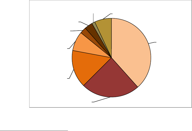
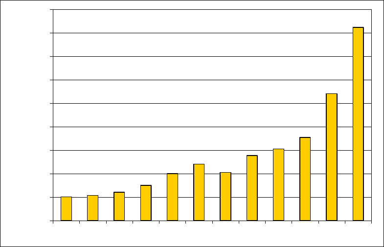
Cumulative installed PV capacity worldwide is 13.9 GW, with data from multiple sources
represented in Figure 1.1 (EurObserv’ER 2009, IEA 2009, Mints et al. 2009, Sherwood/IREC
2009).
1
Germany is the clear leader at 5.3 GW of cumulative installed capacity, followed by
Spain, Japan, the United States, Italy, South Korea, and France. Other European Union (EU)
countries contributed about 0.37 GW of the 0.97 GW attributed to the Rest of World (ROW)
countries.
2
The capacity of 13.9 GW is a 75% increase over 7.9 GW of 2007 cumulative
installed capacity, for a 2008 addition of approximately 6.0 GW. The 6.0 GW represents a 152%
increase over 2.4 GW installed in 2007.
Figure 1.1 Global cumulative installed PV capacity through 2008
(EurObserv’ER 2009, IEA 2009, Mints et al. 2009, Sherwood/IREC 2009)
1
Data for the top countries shown in Figure 1.1 are from IEA 2009. 2008 data for EU countries not included in IEA
2009 are from EurObserv’ER 2009 and contribute to the ROW total. U.S. data are from Larry Sherwood/IREC. The
estimate for ROW installed capacity and market share is based on data from IEA 2009 and EurObserv’ER 2009 for
countries not in the top seven; ROW demand share is from Mints et al. 2009.
2
The IEA 2009 report estimates global cumulative installed PV capacity through 2008 to be 13.4 GW. This is close
to the 13.9 GW shown in Figure 1.1, but Figure 1.1 also includes an overall ROW estimate as described in the
previous footnote.
Germany,
5.3 GW, 38%
Spain,
3.4 GW, 24%
Japan,
2.1 GW, 15%
United States,
1.1 GW, 8%
South Korea,
0.36, 3%
Italy,
0.46 GW, 3%
France,
0.18 GW, 1%
Rest of World,
0.97 GW, 7%
2
The range of estimates for cumulative installed PV capacity worldwide through 2008 is between
13 and 17 GW, with at least two sources at the upper end of the range (REN21 2009, Boas et al.
2009). The higher estimates likely represent cumulative production or shipments of PV cells and
modules. In a rapidly growing industry, it makes sense that cumulative production should be
greater than cumulative shipments, which should be greater than cumulative installed capacity.
Data presented in this report reflect cumulative global production of 18.5 GW from 1997 to
2008, cumulative global shipments of 15.2 GW from 1997 to 2008, and cumulative installed
capacity of 13.9 GW.
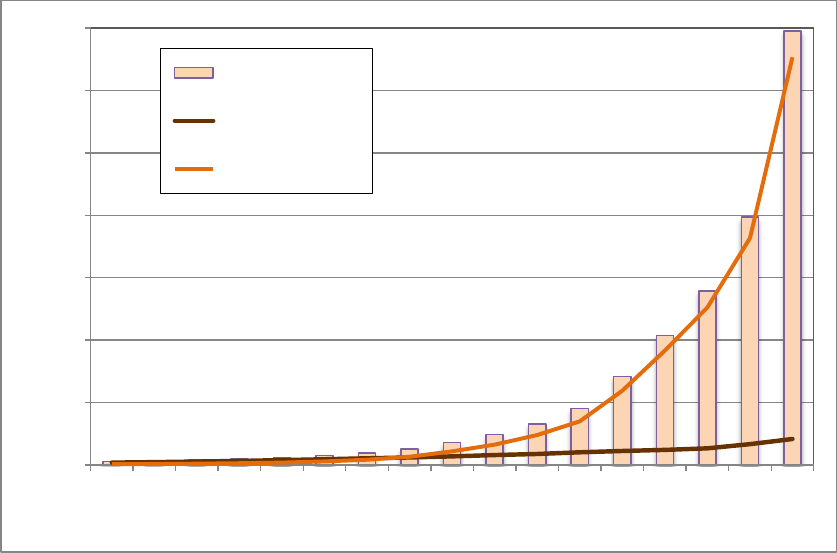
1.1.2 Growth in Cumulative and Annual Installed PV Capacity Worldwide
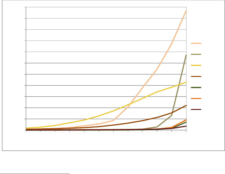
As illustrated in Figure 1.2, Germany’s cumulative installed PV capacity reached 5.3 GW as of
the end of 2008. This is a 38% increase over 2007 cumulative installed capacity of 3.9 GW.
Germany’s market for PV has been supported by a feed-in tariff (FIT) since 2000, providing a
guaranteed payment for a 20-year period for PV-generated electricity feeding into Germany’s
grid. Germany’s PV market experienced its highest annual growth year in 2004, a 290% increase
from 0.15 GW in 2003 to 0.60 GW in 2004, coinciding with an amendment enhancing and
streamlining Germany’s FIT (called Erneuerbare-Energien-Gesetz [EEG]).
3
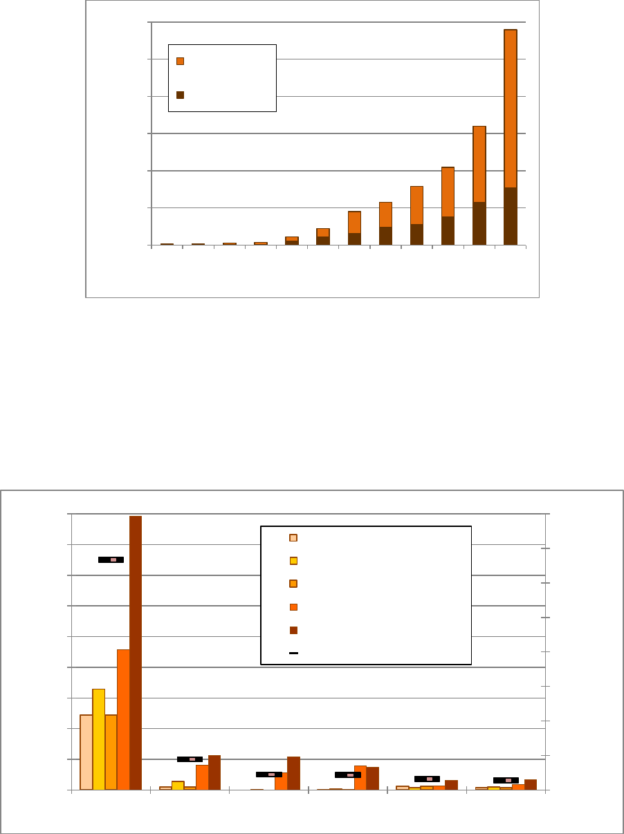
Figure 1.2 Cumulative installed PV capacity in top seven countries
(IEA 2008, IEA 2009, Sherwood/IREC 2009)
3
The revision to the EEG included an overall increase in the per-kWh payment for PV-generated electricity among
other adjustments such as the setting of degression
rates and the specification of payment rates according to PV-
system type (building versus ground mounted) and size.
0.0
0.5
1.0
1.5
2.0
2.5
3.0
3.5
4.0
4.5
5.0
5.5
1997
1998
1999
2000
2001
2002
2003
2004
2005
2006
2007
2008
Cumulative Installed Capacity (GW)
Germany
Spain
Japan
U.S.
Korea
Italy
France
3
Spain surpassed Japan in 2008 as the number two market as measured by cumulative installed
PV capacity of 3.4 GW, a 410% increase over Spain’s 2007 cumulative installed capacity of
0.66 GW. This tremendous increase in capacity was the result of support from Spain’s FIT. This
was the second year that Spain’s cumulative capacity grew by more than 300%. With 2006
cumulative capacity at 0.14 GW, growth to 0.66 MW in 2007 was a 360% increase.
Japan’s cumulative installed capacity reached 2.1 GW in 2008, an approximately 12% increase
over the 2007 level of 1.9 GW. Japan had the largest market for PV until Germany surpassed
Japan in 2005, coinciding with the end of Japan’s “70,000 Roofs” Program. Japan’s cumulative
installed capacity had reached 1.1 GW by the end of 2004, still greater than Germany’s 1.0 GW
at that time.
With U.S. policy support for PV via the federal investment tax credit, as well as state rebate
programs and other incentives and financing mechanisms, the U.S. PV market experienced a
43% increase in cumulative installed capacity, from 0.77 GW in 2007 to 1.1 GW in 2008.
Other leading markets include Italy, South Korea, and France, with 2008 cumulative installed PV
capacity reaching 0.46, 0.36, and 0.18 GW, respectively. This represents growth of 280% for
Italy (0.12 GW in 2007), 360% for South Korea (0.078 GW in 2007), and 140% for France
(0.075 GW in 2007).
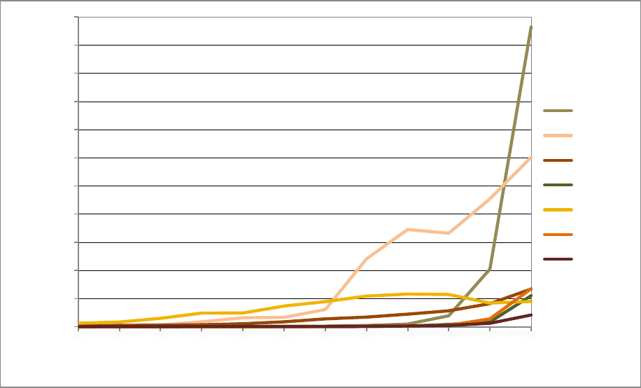
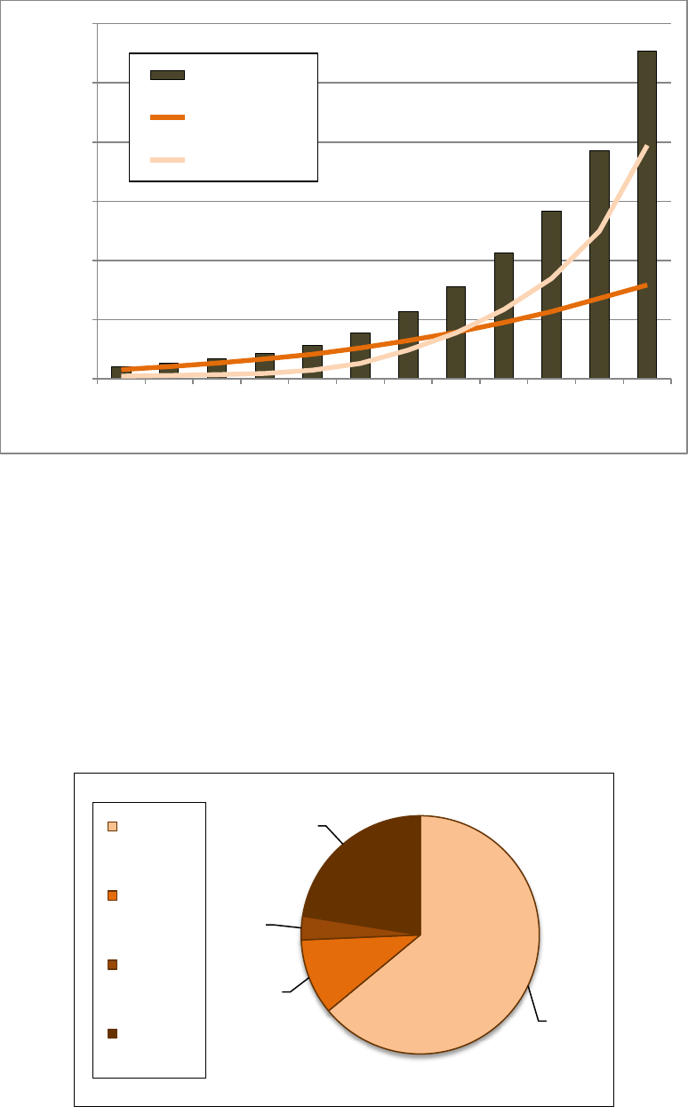
Figure 1.3 presents annual installed PV capacity from 1997–2008 for the seven leading
countries. Spain led in 2008, adding 2.7 GW, an increase of 420% over 0.51 GW installed in
2007. Germany added 1.5 GW in 2008, an increase of 33% (1.1 GW added in 2007). The United
States and Italy were third with 0.34 GW of 2008 additions, a 63% increase for the United States
(0.21 GW added in 2007) and a 380% increase for Italy (0.070 GW added in 2007).
Figure 1.3. Annual installed PV capacity in top seven countries
(IEA 2008, IEA 2009, Sherwood/IREC 2009)
0.00
0.25
0.50
0.75
1.00
1.25
1.50
1.75
2.00
2.25
2.50
2.75
1997
1998
1999
2000
2001
2002
2003
2004
2005
2006
2007
2008
Annual Installed PV Capacity (MW)
Spain
Germany
U.S.
Korea
Japan
Italy
France
4
Other leading markets were South Korea, Japan, and France. South Korea’s annual additions
topped Japan’s, increasing from 0.043 GW in 2007 to 0.28 GW in 2008 (540% growth). Japan
added 0.23 GW, an increase of 7% over the 2007 level of 0.21 GW. France added 0.10 GW in
2008, a 230% increase over the 0.031 GW installed in 2007.
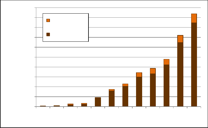
1.1.3 Worldwide PV Installations by Interconnection Status and Application
As illustrated in Figure 1.4, grid-connected PV has represented the majority of installed capacity
additions worldwide since about 1999, increasing its cumulative market share each year: 44% in
1998, 52% in 1999, nearly 92% in 2007, and 94% in 2008. The grid-connected market
contributed 97% of 2008 capacity additions. The faster growth in the grid-connected PV market
has been supported by incentives for grid-connected PV in the top global markets. The grid-
connected market grew at 10- and 5-year CAGRs of 54% and 56%, respectively, while the off-
grid market grew at 10- and 5-year CAGRs of 14% and 15%, respectively.
Grid-connected, cumulative installed capacity represented in Figure 1.4 grew nearly 80% from
7.3 GW in 2007 to 13.1 GW in 2008. Off-grid capacity grew 24% from 0.67 GW in 2007 to
0.83 GW in 2008. Grid-connected markets are typically easier to track than off-grid, because
grid-connected data associated with incentive programs are generally available, whereas off-grid
data are often elusive.
Figure 1.4. Global cumulative installed PV capacity by interconnection status
(EurObserv’ER 2009, IEA 2008, IEA 2009)
0
2
4
6
8
10
12
14
1992
1993
1994
1995
1996
1997
1998
1999
2000
2001
2002
2003
2004
2005
2006
2007
2008
Cumulative Installed Capacity (GW)
Total
Off-grid
Grid-Connected
5
The continued success of Germany’s PV market and the recent high rates of growth in Spain and
Italy are due largely to support in the form of FITs. This production incentive has greatly
motivated the installation of rooftop, grid-connected PV and large PV power plants in Germany,
large-scale PV plants in Spain, and grid-connected distributed generation in Italy (IEA 2008).
Incentives in the United States and other top markets have also greatly favored grid-connected
additions.
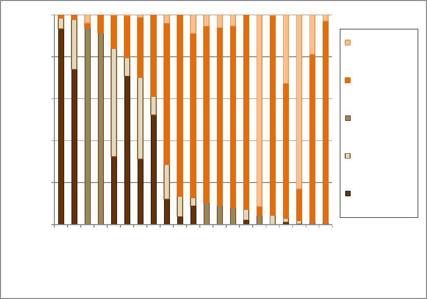
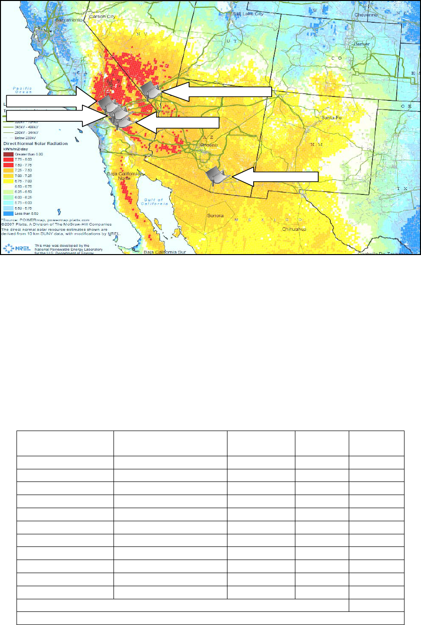
Despite dominance of the grid-connected market worldwide, there is still variation in the types of
PV systems installed in different countries, reflecting various types of subsidy support, market
maturity, demand for particular applications, and various economic and cost factors. More than
half of the countries listed in Figure 1.5 have a majority of grid-connected PV, including
Germany, Spain, Japan, South Korea, Italy, and the United States (toward the right side of the
graph). Cumulative installed capacity for countries such as Sweden, Israel, Malaysia, Turkey,
Mexico, and Norway (shown to the left of the United States on the graph) have a dominant off-
grid residential market. In Canada and Australia, significant portions of the PV markets consist
of off-grid commercial PV installations. In Australia, this capacity consists mainly of off-grid
industrial and agricultural applications (IEA 2009).
Figure 1.5. Application market share of cumulative installed PV capacity
in IEA countries through 2008
(IEA 2009, Mints 2009)
0%
20%
40%
60%
80%
100%
Norway
Mexico
Turkey
Malaysia
Canada
Israel
Australia
Sweden
US
Denmark
France
Austria
Netherlands
Switzerland
Great Britain
Portugal
Japan
Italy
South Korea
Spain
Germany
Market share of cumulative installed PV capacity
Grid-connected
utility
Grid-connected
distributed
Off-grid
undefined
Off-grid
non-domestic
Off-grid
domestic

6
1.2 U.S. Installed PV Capacity
1.2.1 Cumulative U.S. Installed PV Capacity
Cumulative installed PV capacity
4
in the United States topped 1 GW in 2008, increasing 43%
from 0.77 GW in 2007 to 1.1 GW by the end of 2008 (Sherwood/IREC 2009).
5
Enhanced government support on both the federal and state levels has been critical for expanding
the adoption of solar energy in the United States since 2005. The Energy Policy Act of 2005
(EPACT 2005) raised the federal investment tax credit (ITC) for solar from 10% to 30% for
nonresidential installations and from 0% to 30% for residential installations. EPACT 2005
capped the ITC for residential solar installations at $2,000, but this cap was removed by the
Emergency Economic Stabilization Act of 2008 (EESA), effective January 1, 2009. On the state
level, large incentive programs, such as the California Solar Initiative (CSI) and New Jersey’s
Consumer On-site Renewable Energy Program, offered rebates covering a significant proportion
of the up-front costs of PV systems. Other state and local policies, such as renewable portfolio
standards (RPSs) and improved interconnection and net metering rules, have further promoted
the growth of solar energy in recent years.
U.S. PV
installation growth has been accelerating in recent years. The United States installed 0.34 GW in
2008, an annual increase of 63% over 0.21 GW installed in 2007. Growth in annual additions
from 0.14 GW in 2006 to 0.21 GW in 2007 was 44%, and the 5-year CAGR for annual additions
from 2003 to 2008 was 37%.
1.2.2 U.S. PV Installations by Interconnection Status
In the United States, cumulative, installed off-grid PV capacity was higher than grid-connected
capacity until 2004 (Figure 1.6). The grid-connected market has since dominated and continued
to increase its market share (65% in 2007, 71% in 2008), which is due to federal and state
incentive support. Of the 1.1 GW of cumulative installed PV capacity in 2008, an estimated
0.79 GW are grid connected and 0.32 GW are off grid.
4
Includes grid-connected and off-grid installed PV capacity.
5
The U.S. installed PV capacity data presented in this report are based on data from Larry Sherwood, with the full
reference to his report, U.S. Solar Market Trends 2008,
http://irecusa.org/irec-programs/publications-reports/,
provided at the end of Chapter 1. Note that the numbers presented in this chapter are slightly different from those in
Sherwood’s report, as the data used for this report were obtained directly from him in June 2009.
7
Figure 1.6. U.S. cumulative installed PV capacity by interconnection status
(Sherwood/IREC 2009)
1.2.3 U.S. PV Installations by Application and Sector
In addition to grid-connected versus off-grid, PV installations can be categorized by application,
including building-integrated, rooftop, and ground-mounted PV, and sector, which comprises
residential, commercial, and utility markets.
As shown in Figure 1.7, rooftop PV installations were estimated at 64% or nearly two-thirds of
U.S. installations in 2008. Assuming 0.34 GW or about 340 MW installed in the United States in
2008, as stated in Section 1.2.1, rooftop installations amounted to nearly 218 MW.
Figure 1.7. U.S. PV applications, 2008 market shares
(EuPD Research 2008)
0.00
0.20
0.40
0.60
0.80
1.00
1.20
1997
1998
1999
2000
2001
2002
2003
2004
2005
2006
2007
2008
Cumulative Installed Capacity (GW)
Total
Off-Grid
Grid-Connected
64%
10%
3%
22%
Rooftop
Roof-
integrated
Façade-
integrated
Ground-
mounted
8
During the past couple of years, there has been an increase in the installation of ground-mounted
PV systems. The Boulder City, Nevada, 10-MW, ground-mounted PV project, which came
online in December 2008, is the largest thin-film solar power plant in North America. The
project was developed by Sempra Generation and consists entirely of First Solar thin-film
modules (First Solar 2008). Large ground-mounted PV systems were also installed in 2007 at
Nellis Air Force Base in Nevada (14 MW) and Alamosa, Colorado (8 MW). Only one new large
installation came online in 2008, but many new ground-mounted projects began development in
2008. Examples are Pacific Gas & Electric’s 550-MW Topaz Solar Farm and the 250-MW
California Valley Solar Ranch (Bradford et al. 2008). Large PV systems are expected to increase
in market share, supported by the utilities’ need to meet renewable portfolio standard (RPS) and
solar set-aside requirements and their recently legislated ability to utilize the federal ITC
(expanded ITC passed October 2008).
Figure 1.8 shows that although the number of nonresidential installations including commercial
and utility PV is increasing, the residential sector still accounts for the vast majority of annual
installations. In 2008 nearly 17,000 grid-connected residential installations were installed,
compared to fewer than 2,000 grid-connected nonresidential PV installations.
Figure 1.8. Annual trend in number of U.S. grid-connected PV installations by sector
(Sherwood/IREC 2009)
Although grid-connected residential PV installations have greatly outnumbered grid-connected
nonresidential PV installations for almost a decade, the annual capacity added by new
nonresidential PV installations is much greater because of larger system sizes in the commercial
and utility sectors. As indicated in Figure 1.9, the additional capacity from grid-connected
nonresidential installations accounted for 73% of the 0.29 GW (or 290 MW) of grid-connected
capacity added in 2008.
0
2,000
4,000
6,000
8,000
10,000
12,000
14,000
16,000
18,000
20,000
1997
1998
1999
2000
2001
2002
2003
2004
2005
2006
2007
2008
Annual Number of Installations
Nonresidential
Residential
9
Figure 1.9. U.S. annual grid-connected PV capacity
(Sherwood/IREC 2009)
1.2.4 U.S. States with the Largest PV Markets
The top six states in terms of cumulative, installed grid-connected PV capacity as of the end of
2008 were California (530 MW, 67% market share), New Jersey (70 MW, 9% market share),
Colorado (36 MW, 4.5% market share), Nevada (34 MW, 4% market share), Arizona (25 MW,
3% market share), and New York (22 MW, 3% market share).
Figure 1.10. Annual grid-connected PV capacity and cumulative market share
in top U.S. state markets, 2004–2008
(Sherwood/IREC 2009)
0
50
100
150
200
250
300
1997
1998
1999
2000
2001
2002
2003
2004
2005
2006
2007
2008
Annual Installed Capacity (MW)
Nonresidential
Residential
0%
10%
20%
30%
40%
50%
60%
70%
80%
0
20
40
60
80
100
120
140
160
180
California
New Jersey
Colorado
Nevada
Arizona
New York
Cumulative Market Share (%)
Annual Installed Capacity (MW)
2004
2005
2006
2007
2008
Cumulative Market Share

10
Figure 1.10 shows annual installed capacity for the top six states for the past 5 years. California
continued to lead the U.S. market with nearly 180 MW of new grid-connected PV in 2008,
representing 95% growth from the 92 MW installed in 2007. In New Jersey, 23 MW of new
capacity were installed in 2008, amounting to 37% annual growth from the 16 MW installed in
2007. Colorado’s annual capacity additions increased 88% from 11 MW installed in 2007 to
22 MW installed in 2008. Annual installed capacity in Nevada decreased slightly from 16 MW in
2007 to 15 MW in 2008, with most new capacity coming from the 10-MW El Dorado project.
Arizona continued to see steady growth with a 130% increase in installed capacity, from 2.8 MW
in 2007 to 6.4 MW in 2008. In New York, 7 MW were installed in 2008, an 85% increase over
the 3.8 MW installed in 2007.
1.3 Global and U.S. Installed CSP Capacity
1.3.1 Cumulative Installed CSP Worldwide
At the end of 2008, there were 430 MW of cumulative, grid-tied concentrating solar power
(CSP) capacity worldwide, with more than 95% (419 MW) of this global capacity located in the
southwestern United States. By July 2009, global capacity increased to about 550 MW with the
addition of 120 MW in Spain. This reduced the U.S. share to approximately 75%. Of the
550 MW of CSP worldwide, nearly 95% (519 MW) is parabolic trough technology, with the
remainder (31 MW) being tower technology. Table 1.1 lists installed CSP plants worldwide as of
July 2009.
Table 1.1. Global Installed CSP Plants
Plant Name Location Technology Type Year Installed Capacity (MW)
SEGS I - IX
California, United States
Trough
1985–1991
354
APS Saguaro
Arizona, United States
Trough
2005
1
Nevada Solar One
Nevada, United States
Trough
2007
64
PS10
Spain
Tower
2007
11
Puertollano Plant
Spain
Trough
2009
50
Andasol I
Spain
Trough
2009
50
PS20
Spain
Tower
2009
20
Grama et al. 2008
1.3.2 Major non-U.S. International Markets for CSP
Besides the United States, Spain and North Africa are promising markets for CSP. The first
commercial CSP plant in Spain, the 11-MW tower system known as PS10, was completed in
2007. With a 25% capacity factor, PS10 can generate 24 GWh/yr, enough to supply about 5,500
households with electricity (Grama et al. 2008). No new systems were connected to the grid in
Spain in 2008.
As of July 2009, nearly 400 MW of CSP capacity, mostly trough systems, were under
construction in Spain, supported by the government’s feed-in tariff (FIT) policy, which
guarantees payment for electricity produced by a CSP system. The FIT has two major
restrictions. First, the maximum allowable size of a plant is 50 MW. Second, there is an overall

11
capacity ceiling of 500 MW. During the first half of 2009, construction was completed on the
50-MW Andasol I trough plant and the 50-MW Puertollano trough plant (Solar Millennium
2009, CSP Today 2009). Andasol I became the first commercial CSP plant with energy-storage
capability designed specifically for electricity generation after sunset. This added feature enables
the plant to provide electricity for ~7.5 hours after sunset (Solar Millennium 2009).
The region of North Africa has the potential for sizable CSP growth. Feasibility studies show
that North African power plants could provide about 15% of Europe's electricity needs. One of
the requirements for this to occur is the construction of a 2,000-mile transmission cable
connecting the two continents (Merrill Lynch 2008). Discussion on the matter has occurred, but
major policy decisions have yet to be made. In Morocco, 20 MW of CSP will be hybridized with
a natural gas plant (Global Environment Facility 2009), and similar planning is under way in
Algeria and Egypt. This type of design, known as an integrated solar combined cycle (ISCC), is
gaining some traction in the region. An ISCC plant combines heat from the natural gas turbine
and the solar field, achieving capacity gains without increasing emissions. Another benefit of
such a system is that an additional turbine is not needed when the CSP portion is built. This both
speeds up the construction process and helps keep capital expenditures in check.
On the global level, nearly 600 MW of CSP were in the engineering, procurement, and
construction stages by the end of 2008 (Grama et al. 2008), as summarized in Table 1.2. The
majority were trough systems being built in Spain, with North African countries installing trough
and tower capacity as part of ISCC plants. Mexico and China were also constructing trough
systems.
Table 1.2. CSP Plants Under Construction, by Country
Country
Technology Type
Capacity (MW)
Algeria
Trough
43
Australia Linear Fresnel Reflector 1
China
Trough
50
Egypt Tower 31
Mexico
Trough
29
Morocco Trough 30
Spain
Trough
350
Spain Tower 37
Total
571
Grama et al. 2008
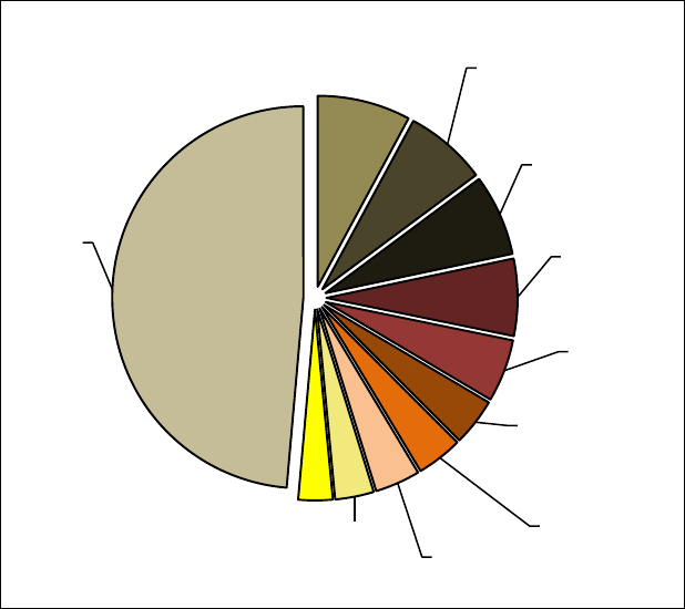
1.3.3 U.S. Installed CSP Capacity
As of the end of 2008, 419 MW of grid-tied CSP capacity had been installed in the southwestern
United States, accounting for more than 95% of global CSP capacity. The Solar Electricity
Generating Stations (SEGS) in the Mojave Desert of southern California account for 354 MW of
this capacity. SEGS comprises nine parabolic trough plants, ranging from 14 to 80 MW, located
in three main locations (Daggett, Harper Lake, and Kramer Junction); this is illustrated in
Figure 1.11. The plants were built between 1984 and 1991 and together have generated more
than 11,000 GWh (BrightSource 2008).
12
Figure 1.11. Concentrating solar power plants of the southwest United States
(NREL 2009)
As summarized in Table 1.3, the next CSP plant to come online in the United States after the
SEGS plants was the Arizona Public Service (APS) Saguaro 1-MW parabolic trough plant.
Installed in Red Rock, Arizona, in 2005, the system has a capacity factor of 23%, allowing for
the generation of 2 GWh per year (Grama et al. 2008). Another 64 MW of CSP capacity are
accounted for by the Nevada Solar One parabolic trough plant in Boulder City, Nevada.
Connected to the grid in 2007, this plant has a capacity factor of 23% and generates more than
130 GWh each year (Acciona Energy 2008, Grama et al. 2008). The estimated cost of electricity
generated by the Nevada Solar One plant is about $0.18/kWh (Bullard et al. 2008).
Table 1.3. Installed CSP Plants in the United States
Plant Name
Location
Technology
Type
Year
Installed
Capacity
(MW)
SEGS I
Daggett, CA
Trough
1985
14
SEGS II
Daggett, CA
Trough
1986
30
SEGS III
Kramer Junction, CA
Trough
1987
30
SEGS IV
Kramer Junction, CA
Trough
1987
30
SEGS V
Kramer Junction, CA
Trough
1988
30
SEGS VI
Kramer Junction, CA
Trough
1989
30
SEGS VII
Kramer Junction, CA
Trough
1989
30
SEGS VIII
Harper Lake, CA
Trough
1990
80
SEGS IX
Harper Lake, CA
Trough
1991
80
APS Saguaro
Saguaro, AZ
Trough
2005
1
Nevada Solar One
Boulder City, NV
Trough
2007
64
Total
419
Grama et al. 2008
Nevada Solar One, 64MW
APS Saguaro, 1MW
SEGS III-VII, 150MW
SEGS I & II, 44 MW
SEGS VIII & IX, 160MW

13
1.4 References
Acciona Energy. (2008). www.acciona-na.com/. Accessed November 2008.
Boas, R.; Farber, M.; Flynn, H.; Meyers, M.; Porter, C.; Rogol, M.; Song, J. (March 2009).
Photon International. “Looking back—sizing the 2008 solar market.” pp. 88–93.
Bradford, T.; Englander, D.; Maycock, P. (June 2008). “The Growth of Utility Scale PV.” PV
News. Prometheus Institute and Greentech Media.
BrightSource Energy, Inc. (2008). www.brightsourceenergy.com/bsii/history/. Accessed
November 2008.
Bullard, N.; Chase. J.; d’Avack, F. (May 20, 2008). “The STEG Revolution Revisited.” Research
Note. London: New Energy Finance.
CSP Today. (May 12, 2009). “Iberdrola launches its first solar thermal power plant.” Weekly
Intelligence Brief. www.csptoday.com/. Accessed May 2009.
EuPD Research. (2008). Photovoltaics in the USA: Detailed Analysis of a future solar market,
management summary. Bonn, Germany: EuPD.
EurObserv’ER. (2009). Photovoltaic Barometer. Paris, France: EurObserv’ER Consortium.
http://www.eurobserv-er.org/downloads.asp. Accessed July 2009.
First Solar Inc. (December 22, 2008). “First Solar Completes 10MW Thin Film Solar Power
Plant for Sempra Generation.” News Release.
http://investor.firstsolar.com/phoenix.zhtml?c=201491&p=irol-
newsArticle&ID=1238556&highlight=. Accessed November 25, 2009.
Global Environment Facility. (2009). GEF Project Database.
http://gefonline.org/projectDetailsSQL.cfm?projID=647. Accessed July 2009.
Grama, S.; Wayman, E.; Bradford, T.; (2008) Concentrating Solar Power—Technology, Cost,
and Markets. 2008 Industry Report. Cambridge, MA: Prometheus Institute for Sustainable
Development and Greentech Media.
International Energy Agency (IEA). (2008). Trends in photovoltaic applications: Survey report
of selected IEA countries between 1992 and 2007. Report IEA-PVPS T1-17: 2008. IEA
Photovoltaic Power Systems Programme (PVPS). http://www.iea-pvps.org/ Accessed February
2009.
International Energy Agency (IEA). (2009). Trends in photovoltaic applications. Survey report
of selected IEA countries between 1992 and 2008. Report IEA PVPS T1-18:2009. IEA
Photovoltaic Power Systems Programme (PVPS). http://www.iea-pvps.org/ Accessed November
2009.
Merrill Lynch. (2008). Solar Thermal: Not Just Smoke and Mirrors. New York, NY: Merrill
Lynch.
Mints, P.; (2009). Analysis of Worldwide Markets for Photovoltaic Products and Five-Year
Application Forecast 2008/2009. Report # NPS-Global4. Palo Alto, CA: Navigant Consulting
Photovoltaic Service Program.
Mints, P.; Pogrebnyak, L.; Burmon, A. (February 23, 2009). “Bimonthly Photovoltaic Industry
Update.” Solar Outlook. Issue SO2009-1. Palo Alto, CA: Navigant Consulting, Inc.

14
NREL. (2009). “Concentrating solar power plants of the southwest United States.” Golden, CO:
National Renewable Energy Laboratory (internal only).
Renewable Energy Policy Network for the 21
st
Century (REN21). (2009). Renewables Global
Status Report 2009 Update. Paris, France: REN21 Secretariat. www.ren21.net/publications.
Accessed July 2009.
Sherwood, L. (2009). U.S. Solar Market Trends 2008. Latham, NY: Interstate Renewable Energy
Council (IREC). http://irecusa.org/irec-programs/publications-reports/. Accessed August 2009.
Solar Millennium. (July 1, 2009). ”Andasol I is officially inaugurated.” Press Release.
http://www.solarmillennium.de/Press/Press_Releases/Andasol_1_is_officially_inaugurated,lang2
,50,1660.html. Accessed August 2009.

15
2. Industry Trends, Photovoltaic and Concentrating Solar Power
This chapter covers global and U.S. PV and CSP industry trends. Section 2.1 summarizes global
and U.S. PV cell/module production trends, including production levels, growth over the past
decade, and top producers. Section 2.2 presents data on global and U.S. PV cell/module
shipments and associated revenue, including shipment levels and growth over the past decade,
top companies in terms of shipments, shipment levels by type of PV technology, and U.S. import
and export data. Section 2.3 provides information on major CSP component manufacturers and
CSP component shipments. Section 2.4 discusses material and supply-chain issues for PV and
CSP, including polysilicon, rare metals, and glass supply for PV; material and water constraints
for CSP; and land and transmission constraints for utility-scale solar projects. Section 2.5 covers
global and U.S. solar industry employment trends for both PV and CSP.
2.1 PV Production Trends
2.1.1 Global PV Production
The global PV industry has seen impressive growth rates in cell/module production during the
past decade, with a 10-year CAGR of 46% and a 5-year CAGR of 56% through 2008. Annual
growth from 2007 to 2008 was 87%, higher than the 51% annual growth from 2006 to 2007.
Global production (Figure 2.1) reached 6.9 GW for the year 2008, an 87% increase over 3.7 GW
produced in 2007, which was led primarily by manufacturers in Europe, China, and Japan. The
market shares for the top regions/countries are 27% each for Europe and China, 18% for Japan,
12% for Taiwan, 6% for the United States, and 10% for the rest of the world (ROW). From 1997
to 2008, approximately 18.5 GW of PV cells were produced globally.
Figure 2.1. Global annual PV cell/module production by region
(Maycock 2002, Bradford et al. 2006, Bradford et al. 2008a, Bradford et al. 2009)
0.0
0.5
1.0
1.5
2.0
2.5
3.0
3.5
4.0
4.5
5.0
5.5
6.0
6.5
7.0
1997
1998
1999
2000
2001
2002
2003
2004
2005
2006
2007
2008
Annual PV cell/module production (GW)
ROW
Taiwan
China
Europe
Japan
U.S.
16
Europe and Japan have had strong production growth rates during the past decade, with 10-year
CAGRs of 50% and 38% (from 1998–2008), respectively, resulting in their dominance of the PV
market. Europe and Japan increased their collective market share from 24% in 1980 to 76% in
2004. Since 2004, however, their combined share has dropped to approximately 45%, which is
due to the rapid growth of emerging producers such as China and Taiwan.
China has seen the highest growth rates in recent years, with a 5-year (2003–2008) CAGR of
170%. In 2001, China contributed only about 1% of global production; it did not become a
significant global contributor until 2005 when its market share reached 7%. Taiwan has also
experienced high growth rates, with a 5-year CAGR of approximately 119%, surpassing U.S.
production levels in 2007 to become the world’s fourth-largest producer. Taiwan continued to
gain market share over the United States in 2008. Production in Taiwan increased from
approximately 0.37 GW (10% market share) in 2007 to 0.85 GW (12% market share) in 2008.
The United States produced 0.27 GW (7% market share) in 2007 and 0.41 GW (6% market
share) in 2008.
Figure 2.2 shows 2008 market shares for the top ten PV cell/module producers worldwide, and
Figure 2.3 shows production data for the top ten companies from 2002 to 2008. Japan-based
Sharp Corporation was the global leader in PV production between 2000 and 2006. In 2007,
German-based Q-cells overtook Sharp to become the world’s number-one producer at 0.39 GW
and maintained this position through 2008. Sharp’s market share for production continued to
decrease through 2008, dropping from 9% in 2007 to 6% in 2008. Q-cells also lost production
market share, dropping from 11% in 2007 to 8% in 2008.
Figure 2.2. Top global PV cell/module producers 2008
(Bradford et al 2009)
Q-Cells
0.57 GW
8%
First Solar
0.50 GW
7%
Suntech
0.50 GW
7%
Sharp
0.47 GW
6%
Motech
0.38 GW
5%
Kyocera
0.29 GW
4%
Baoding
Yingli
0.28 GW
4%
JA Solar
0.28 GW
4%
SunPower
0.24 GW
3%
Sanyo
0.21 GW
3%
Other
3.5 GW
49%

17
Figure 2.3. Global annual PV cell/module production by manufacturer 2002–2008
(Bradford et al. 2006, Bradford et al. 2008a, Bradford et al. 2009)
Q-cells, a crystalline and thin-film cell producer, has seen impressive growth rates since 2003
when it first became one of the top-ten producers. Q-cells had a 5-year (2003–2008) CAGR of
about 83%. The German company’s 2008 production was 47% greater than its 2007 production
of 0.39 GW. Although Q-cells has all of its manufacturing plants in Germany, its plans for future
expansion include development of overseas capacity in places such as Malaysia.
First Solar is a U.S. company with production facilities in the United States, Germany, and
Malaysia. First Solar became a top-ten producer for the first time in 2007 and maintained this
position through 2008. This marked the first time a predominantly thin-film manufacturer made
the top-ten list. First Solar, the largest U.S. PV cell/module manufacturer, was responsible for
36% of total U.S. production in 2008. First Solar is the world’s largest manufacturer of thin-film
(CdTe) modules with 0.15 GW of production in the United States, 0.20 GW of production in
Germany, and 0.16 GW of production in Malaysia in 2008. First Solar’s jump in the global
rankings is a result of high growth rates in recent years. Its 2008 production level grew to
0.50 GW in 2008, up 740% from the 2006 level. First Solar expects its capacity to exceed 1 GW
by the end of 2009. In addition to impressive production numbers, First Solar also boasted the
PV industry’s lowest cell manufacturing cost of $1.08/W in the third quarter of 2008 (First Solar
2008).
Suntech Power, a Chinese crystalline silicon company with production in China, was the third-
largest PV producer in 2008. The company has seen impressive growth rates in recent years,
producing 0.50 GW in 2008, up from 0.33 GW in 2007.
Sharp Corporation also has plans for growth. The Japanese company’s 2008 manufacturing
capacity was 0.86 GW, with most being crystalline cells. The company, however, plans to shift
0.0
1.0
2.0
3.0
4.0
5.0
6.0
7.0
8.0
2002 2003 2004 2005 2006 2007 2008
Annual PV cell/module production (GW)
Sanyo
SunPower
JA Solar
Baoding Yingli
Kyocera
Motech
Sharp
Suntech
First Solar
Q-Cells
Other
18
its focus from crystalline technologies to thin-film PV going forward. Sharp indicated it plans to
upgrade its current 15-MW, thin-film plant to a 160-MW plant. The company is also developing
a 1-GW, thin-film plant within a liquid crystal display (LCD) manufacturing facility. Sharp
estimates that the new factory will begin thin-film shipments in 2010.
Motech Solar, a crystalline silicon cell producer, is the largest PV producer in Taiwan and the
sixth largest globally. The company’s 2008 production of 0.38 GW is a 120% increase over its
2007 production value of 0.18 GW. Motech has indicated plans to expand its PV production
capabilities into China and the United States.
2.1.2 U.S. PV Production
As with the global trend in PV production, the United States has seen strong growth rates in the
past decade, with a 10-year CAGR of 23% and a 5-year CAGR of 32%. Production in 2008
reached 0.41 GW, an increase of 52% over 0.27 GW produced in 2007. Figure 2.4 illustrates
production levels from 1997–2008. In 2003, the U.S. PV industry experienced an 18-MW dip in
production, resulting primarily from the bankruptcy of AstroPower, the second-largest U.S.
producer at that time. AstroPower’s 30-MW production capacity and assets were acquired by GE
Energy for $15 million. After 2003, U.S. production resumed strong growth. Despite increases in
domestic production, U.S. market share in global production has fallen to 6%, which is due to
more rapid growth in other regions/countries such as Europe, China, and Taiwan. The United
States dominates global thin-film production.
Figure 2.4. U.S. annual PV cell/module production
(Maycock 2002, Bradford et al. 2006, Bradford et al. 2008a, Bradford et al. 2009)
Figures 2.5 and 2.6 summarize U.S. annual PV cell/module production by manufacturer.
0.00
0.05
0.10
0.15
0.20
0.25
0.30
0.35
0.40
0.45
1997
1998
1999
2000
2001
2002
2003
2004
2005
2006
2007
2008
Annual PV cell/module production (GW)
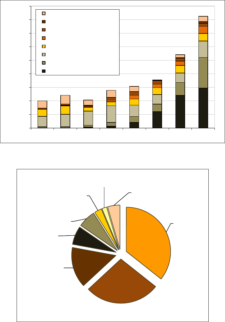
19
Figure 2.5. U.S. annual PV cell/module production by U.S. manufacturer
(Bradford et al. 2006, Bradford et al. 2008a, Bradford et al. 2009)
Figure 2.6. Top U.S. PV cell/module producers 2008
(Bradford et al. 2009)
The United States is the global leader in thin-film PV cell/module production, and accordingly,
the top two U.S. manufacturers for 2008 were both thin-film producers. Thin-film PV
cells/modules produce electricity via extremely thin layers of semiconductor material made of
0.00
0.05
0.10
0.15
0.20
0.25
0.30
0.35
0.40
0.45
2001
2002
2003
2004
2005
2006
2007
2008
Annual PV cell/module production (GW)
Other
Global Solar
Schott Solar
Evergreen Solar
BP Solar
Solarworld CA (Shell Solar)
United Solar Ovonics
First Solar
First Solar,
147 MW,
36%
United Solar
Ovonics,
113 MW,
27%
Solarworld
CA (Shell
Solar),
61 MW,
15%
BP Solar,
28 MW, 7%
Evergreen
Solar,
27 MW, 6%
Schott Solar,
11 MW, 3%
Global Solar,
7 MW, 2%
Other
4%
20
cadmium telluride (CdTe), amorphous silicon (a-Si), copper indium gallium diselenide (CIGS),
copper indium diselenide (CIS), or other emerging materials. First Solar is the world’s largest
manufacturer of thin-film (CdTe) modules, with 2008 global production of 0.50 GW, an increase
of 140% from 2007. U.S. production for First Solar in 2008 was 0.15 GW (shown in Figure 2.6
as 147 MW). United Solar Ovonics (or Uni-Solar), a producer of a-Si thin-film technology, was
the second-largest PV producer in the United States in 2008, with a 27% U.S. production market
share. Uni-Solar’s 2008 domestic production reached 110 MW, a 140% increase over its 2007
production level.
In 2008, SolarWorld and BP Solar were ranked third and fourth, respectively, in terms of U.S.
PV production. SolarWorld and BP Solar produced 61 and 28 MW, respectively, in 2008.
Evergreen Solar, fifth in U.S. market share, produced 27 MW in 2008, opened an 80-MW
facility in June 2008, and expects an additional 80-MW capacity at the facility to be completed
in 2009. Schott Solar was ranked sixth, producing 11 MW in 2008. Of Schott Solar’s 80 MW of
global production in 2008, most (88% or 70 MW) were manufactured in Germany. Global Solar,
an Arizona-based company, produced 7.2 MW in 2008; the company primarily manufactures
flexible, thin-film, CIGS-based cells.
2.2 Global and U.S. PV Shipments and Revenue
2.2.1 Global PV Shipments
Shipments of PV cells/modules more accurately reflect demand for PV, as not all cells/modules
end up in the market the year they are produced. Conversely, inventory (produced in an earlier
year) may get shipped out, making it possible for shipments to exceed production in a particular
year and/or for a particular manufacturer. This section presents shipment as opposed to
production data, but does not attempt to compare and reconcile these numbers.
Global shipments of PV cells/modules have seen extensive growth over the last decade, with a
10-year CAGR of 45% and 5-year CAGR of 52% through 2008 (Mints and Tomlinson 2007,
Mints and Tomlinson 2008, Mints 2009). Annual growth from 2007 to 2008 was 79%, higher
than the 55% annual growth from 2006 to 2007.
Global shipments reached 5.5 GW for the year 2008, an increase of 79% from 3.1 GW shipped
in 2007 (Figure 2.7). The market shares for the top regions/countries were 31% for Europe, 22%
for Japan, 19% for China, 11% for Taiwan, 7% for the United States, and 9% for the ROW.
From 1997–2008, a total of approximately 15.2 GW of PV cells/module were shipped globally.
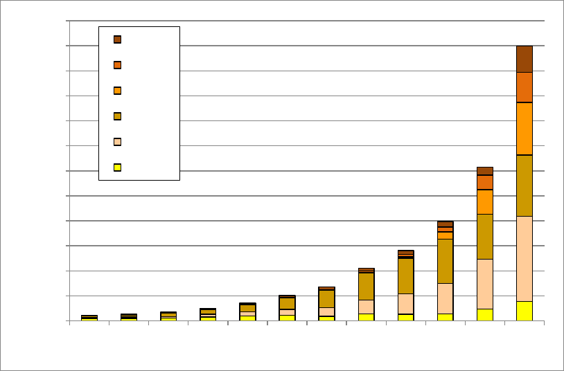
21
Figure 2.7. Global annual PV cell/module shipments by region
(Mints and Tomlinson 2007, Mints and Tomlinson 2008, Mints 2009)
Europe and Japan have achieved significant growth in PV shipments with 10-year CAGRs of
51% and 42% (from 1998–2008), respectively. Shipments in 2008 represented increases of 71%
for Europe (1.7 GW shipped in 2008) and 36% for Japan (1.2 GW in 2008) over 2007 shipment
levels. Europe and Japan increased their joint market share from 47% in 1993 to 80% in 2005.
Since 2005, however, despite continued growth in shipments, the combined Europe and Japan
market share decreased to 53% in 2008, which is due to even more rapid growth of
manufacturers in China and Taiwan.
China has seen a 4-year CAGR of 230% since 2004. China shipped 1.0 GW in 2008, a 110%
increase from 2007. Taiwan has seen similarly impressive growth with a 4-year CAGR of 110%
since 2004. Taiwan shipped 0.61 GW in 2008, a 110% increase from 2007. In 2006, China’s
shipments surpassed those of the United States to become the third-largest contributor to global
PV shipments. In 2007, Taiwan surpassed the United States to become the fourth-largest
contributor. Both China and Taiwan continue to gain market share over the United States. While
the U.S. market share has declined from 9% in 2005 to 7% in 2008, China and Taiwan have
increased their market shares from 2% and 3% in 2005 to 19% and 11% in 2008, respectively.
Figures 2.8 and 2.9 show 2008 PV shipments for the top global manufacturers. In 2008, the
shipments of two companies, BP Solar and Mitsubishi Electric, were statistically close enough to
warrant inclusion in the top 11 manufacturers. In recent years, Sharp Corporation has been the
leading exporter of PV cells/modules. In 2008, however, Q-Cells overtook Sharp with 0.55 GW,
a 59% increase from 2007. SunTech also overtook Sharp as the second leading exporter with
0.50 GW, a 61% increase from 2007. Sharp shipped 0.46 GW in 2008, a 26% increase from
0.0
0.5
1.0
1.5
2.0
2.5
3.0
3.5
4.0
4.5
5.0
5.5
6.0
1997
1998
1999
2000
2001
2002
2003
2004
2005
2006
2007
2008
Annual PV cell/module shipments (GW)
ROW
Taiwan
China
Japan
Europe
U.S.
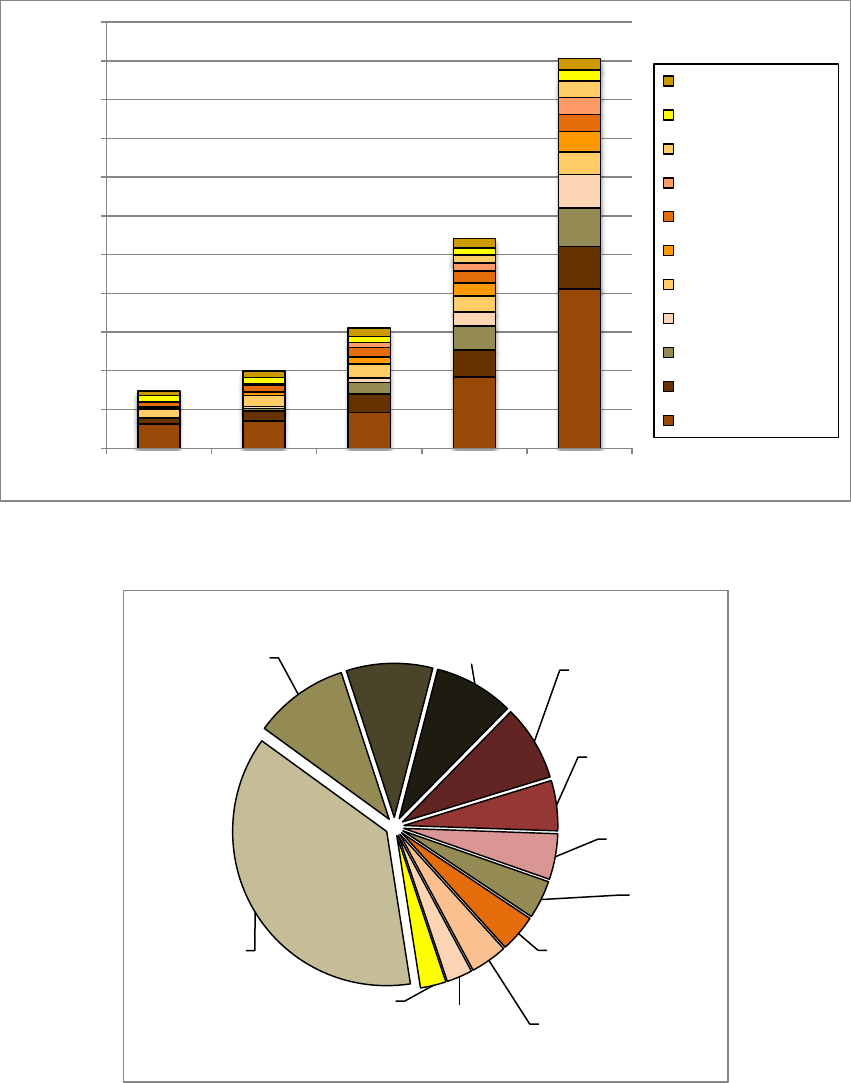
22
2007. In 2007, Sharp experienced a 16% decrease in shipments, a drop from 0.43 GW in 2006 to
0.36 GW in 2007. From 2006 to 2008, Sharp’s growth in shipments totaled 5%.
Figure 2.8. Global annual PV cell/module shipments by manufacturer 2004–2008
(Mints and Tomlinson 2008, Mints 2009)
Figure 2.9. Top global companies for PV cell/module shipments 2008
(Mints 2009)
0.0
0.5
1.0
1.5
2.0
2.5
3.0
3.5
4.0
4.5
5.0
5.5
2004
2005
2006
2007
2008
Annual PV cell/module shipments (GW)
Mitsubishi Electric
BP Solar
JA Solar
Sunpower
Sanyo
Motech
Kyocera
First Solar
Suntech
Q-Cells
Other
Q-Cells,
0.55 GW,
10%
Suntech,
0.50 GW,
9%
Sharp,
0.46 GW,
8%
First Solar,
0.44 GW,
8%
Kyocera ,
0.29 GW,
5%
Motech,
0.26 GW,
5%
Sanyo,
0.22 GW,
4%
SunPower,
0.22 GW,
4%
JA Solar,
0.21 GW,
4%
BP Solar,
0.15 GW,
3%
Mitsubishi
Electric,
0.15 GW,
3%
Other,
2.1 GW,
37%
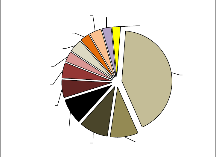
23
First Solar, the world’s leading manufacturer of thin-film PV (specifically CdTe) has
experienced tremendous growth in recent years and overtook Kyocera as the fourth-largest
contributor to global shipments in 2008. First Solar shipped 0.44 GW in 2008, a 130% increase
from 2007. SunPower and JA Solar also experienced significant growth, both with about 110%
increases in shipping from 2007, with 0.22 and 0.21 GW shipped, respectively. The top three
manufacturers, Q-Cells, SunTech, and Sharp, declined in their market shares from 2007 resulting
from the rapid growth of other companies such as First Solar, SunPower, and JA Solar . Q-Cells
declined in market share from 11% in 2007 to 10% in 2008. Similarly, SunTech declined from
10% to 9% and Sharp from 12% to 8%. First Solar increased its market share from 6% in 2007 to
8% in 2008. Both SunPower and JA Solar increased their market shares from 3% in 2007 to 4%
in 2008.
2.2.2 Global PV Cell/Module Revenue
Worldwide revenue from PV cells/modules reached $20 billion in 2008, an increase of 80% from
2007 revenue of $11 billion (Mints 2009). Figure 2.10 provides revenue and associated data for
the top ten global contributors to PV shipments. Q-Cells, Suntech, and Sharp each brought in
close to $2 billion in cell and module revenue in 2008. These three companies each shipped from
nearly 0.46 to 0.55 GW in 2008.
Figure 2.10. Top global companies for PV cell/module revenues 2008
(Mints 2009, company Web sites)
Although there are many types of PV technologies, crystalline silicon cells/modules currently
dominate the world market (Figure 2.11). However, the crystalline silicon market share dropped
slightly in recent years from a 93% share in 2006 to 86% in 2008. Polycrystalline cells currently
Q-Cells,
$1.8 B, 9%
Suntech,
$1.9 B, 9%
Sharp, $1.7 B,
9%
First Solar,
$1.2 B, 6%
Kyocera,
$1.0 B, 5%
Motech,
$0.70 B, 3%
Sanyo,
$0.87 B, 4%
Sunpower,
$0.61 B, 3%
JA Solar,
$0.80 B, 4%
BP Solar,
$0.60 B, 3%
Mitsubishi
Electric,
$0.55 B, 3%
Other,
$8.6 B,
42%

24
lead the global market with a 49% share of total shipments, followed by monocrystalline cells at
35% of shipments.
Globally, thin-film technologies have grown at a 10-year CAGR of 86% from 1998 to 2008. In
2003, the total market share of thin-film cells was 5% compared to the 95% market share of
crystalline cells. In 2008, thin-film technology claimed a 14% global market share (5% a-Si,
8% CdTe, and 1% other thin films). Forecasts of thin-film market share in 2012 have spanned a
broad range, from 16%–34% (see Section 5.3).
Figure 2.11. Global annual PV cell/module shipments by PV technology 1997–2008
(Mints and Tomlinson 2007, Mints and Tomlinson 2008, Mints 2009)
2.2.3 U.S. PV Shipments
During the past decade, the United States has seen steady growth in PV shipments analogous to
the global PV shipment trends, with a 10-year CAGR of 22% and a 5-year CAGR of 33%
through 2008. Figure 2.12 illustrates the annual growth of PV shipped from the United States. In
2003, shipments experienced a 15% dip from the 2002 level, which was due primarily to the
bankruptcy of AstroPower. In 2004, however, the United States experienced a rapid recovery and
increased shipping levels to 30% greater than 2002 values. From 2004 to 2006, the United States
maintained an average of 0.14 GW in shipments each year. After 2006, however, the United
States returned to a state of steady growth. In 2008, 0.39 GW were shipped, a 64% increase from
the 0.24 GW in 2007. In 2008, the United States was the fifth-greatest contributor (by
region/country) to PV shipments with a 7% market share.
0.0
1.0
2.0
3.0
4.0
5.0
6.0
1997 1998 1999 2000 2001 2002 2003 2004 2005 2006 2007 2008
Annual PV cell/module shipments (GW)
CdTe, CIGS, CIS
Amorphous Silicon
Ribbon Silicon
Monocrystalline Silicon
Polycrystalline Silicon
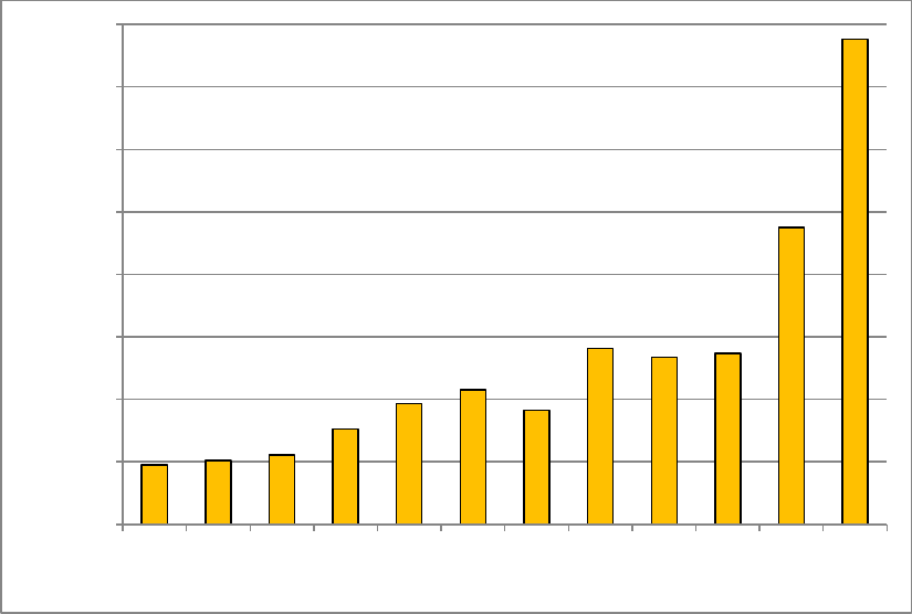
25
Figure 2.12. U.S. annual PV cell/module shipments 1997–2008
(Mints and Tomlinson 2007, Mints and Tomlinson 2008, Mints 2009)
Similar to PV production (described in Section 2.1.2), the two leading U.S. PV shippers in 2008
were thin-film manufacturers. First Solar was the leading U.S. contributor to 2008 shipments
with a 37% market share, or 145 MW, down from a market share of 46% (120 MW) in 2007 (see
Figures 2.13 and 2.14). United Solar Ovonics or Uni-Solar, an a-Si thin-film producer, had the
second-largest market share of U.S. PV shipments in 2008 with a 29% market share,
corresponding to 112 MW. Uni-Solar increased its shipments 130% from its 2007 level, resulting
in a market share increase from 20% in 2007 to 29% in 2008. Other significant contributors to
U.S. PV shipments in 2008 were: Evergreen (17%, 66 MW), BP Solar (9%, 35 MW), Schott
Solar (3%, 11 MW), and SolarWorld (3%, 10 MW). Evergreen jumped from the fifth- to the
third-largest contributor to U.S. shipments by increasing shipment levels 300% in 2008.
0.00
0.05
0.10
0.15
0.20
0.25
0.30
0.35
0.40
1997
1998
1999
2000
2001
2002
2003
2004
2005
2006
2007
2008
Annual PV cell/module shipments (GW)
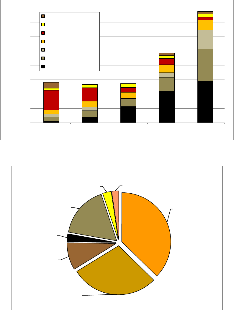
26
Figure 2.13. U.S. annual PV cell/module shipments by manufacturer 2004–2008
(Mints and Tomlinson 2008, Mints 2009)
Figure 2.14. Top U.S. companies for PV cell/module shipments 2008
(Mints 2009)
2.2.4 U.S. PV Cell/Module Revenue
U.S. revenue from PV cells/modules reached $1.2 billion in 2008, an increase of about 46% from
2007 revenue of $0.68 billion (Mints 2009). As shown in Figure 2.15, among U.S. companies in
2008, First Solar had the highest revenue at about $0.35 billion in PV cell/module sales, and
0
50
100
150
200
250
300
350
400
2004
2005
2006
2007
2008
Annual PV cell/module shipments (MW)
Other
Schott Solar
SolarWorld
BP Solar
Evergreen
United Solar Ovonics
First Solar
First Solar ,
145 MW, 37%
Uni-Solar ,
112 MW, 29%
BP Solar ,
35 MW, 9%
SolarWorld,
10 MW, 3%
Evergreen ,
66 MW, 17%
Schott Solar ,
11 MW, 3%
Other, 9 MW,
2%
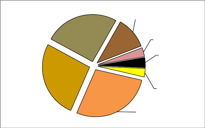
27
United Solar Ovonics (Uni-Solar) had the second highest at $0.33 billion. First Solar is also one
of three U.S.-based companies, including BP Solar and SolarWorld CA, with more than 20 years
of PV production experience. First Solar and BP also earned significant additional revenue from
non-cell or module sales, amounting to an additional $0.20 and $0.09 billion, respectively, in
2008. Four out of seven of the top U.S. PV producers are publicly owned, including First Solar,
Uni-Solar, SolarWorld, and Evergreen Solar. BP, Schott, and Global are all privately owned
solar PV production companies.
Figure 2.15. Top U.S. companies for PV cell/module revenues 2008
(Mints 2009)
2.2.5 U.S. PV Imports and Exports
Figure 2.16 presents data on U.S. PV cell/module imports and exports, including the crystalline
silicon and thin-film contributions. From 1999 to 2004, U.S. PV cell/module exports exceeded
imports significantly. This changed in 2005, when exports and imports nearly evened out,
resulting from increased U.S. imports of crystalline silicon modules and cells and somewhat
offset by increased U.S. exports of thin-film modules/cells. In 2006 and 2007, U.S. total PV
cell/module imports exceeded exports for the first time. Although U.S. thin-film exports doubled
each year from 2005 to 2007, dominating U.S. exports in 2007, U.S. crystalline silicon
module/cell imports grew to more than double the exports in 2006 and 2007. The large increase
in U.S. crystalline silicon module/cell imports was due to a rapid increase in demand for PV
modules and cells, which was particularly high in 2006 in response to the federal investment tax
credit for PV systems included in the Energy Policy Act of 2005. U.S. crystalline PV exports
have remained fairly flat, with increases in exports accounted for by the fast-growing, thin-film
industry.
First Solar,
$0.35 B, 28%
United Solar
Ovonics,
$0.33 B, 26%
Evergreen
Solar,
$0.32 B, 25%
BP Solar,
$0.14 B, 11%
Schott Solar,
$0.039 B, 3%
SolarWorld CA
(Shell Solar),
$0.043 B, 4%
Other,
$0.036 B, 3%
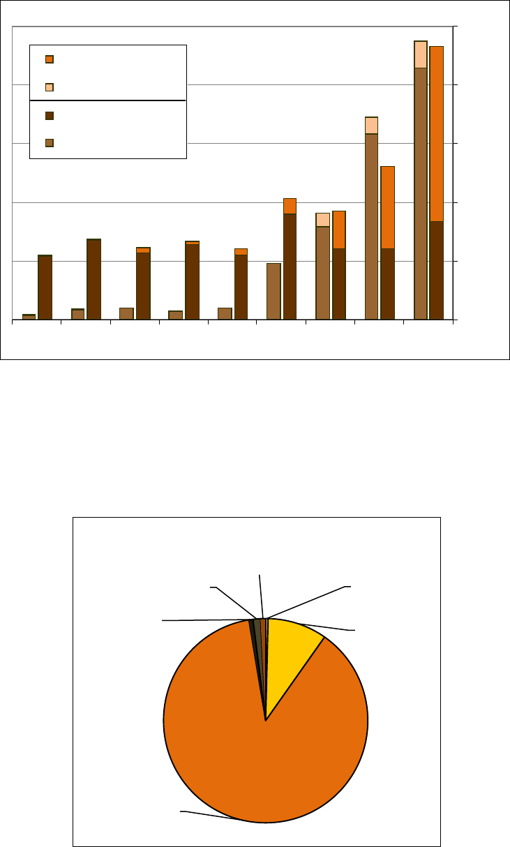
28
Figure 2.16. U.S. PV cell/module shipments, exports and imports
(EIA 2008a)
In 2007, 88% of U.S. PV exports were destined for Europe and 9% went to Asia (Figure 2.17).
The dominance of the European market is due primarily to significant government incentives in
countries such as Germany and Spain, which received about 64% and 13% of U.S. shipments,
respectively.
Figure 2.17. U.S. exports of PV cells and modules, 2007 destination
(EIA 2008a)
1999 2000 2001 2002 2003 2004 2005 2006 2007
0.00
0.05
0.10
0.15
0.20
0.25
GW
Exports Thin Film
Imports Thin Film
Exports Crystalline Si
Imports Crystalline Si
Africa,
0.4%
Asia, 9.4%
Europe,
88%
North &
Central
America,
0.7%
Oceania &
Australia,
1.2%
South
America,
0.8%

29
2.3 CSP Manufacturer and Shipment Trends
Reflectors, receivers, and turbines are the three major components in CSP technologies that are
currently being installed worldwide.
2.3.1 CSP Manufacturers
Table 2.1 lists major CSP component (reflector, receiver, and turbine) manufacturers.
Historically, Flabeg has been the major manufacturer of reflectors, providing a product with 95%
or better reflectivity. Other emerging companies, such as PPG Industries and Rioglass, aim to
lower capital costs of glass and increase durability. Furthermore, other companies (e.g.,
Reflectech, 3M, and Alanod) are offering a reflective film as a lower-cost alternative to
traditional mirrors (Grama et al. 2008). In terms of receivers, Solel has historically been the
major manufacturer, but Schott Solar Systems recently has become a significant player. For
turbines, ABB, GE-Thermodyn, and Siemens are major manufacturers, and companies such as
Alstom, MAN Turbo, and ORMAT are looking to gain market share.
Table 2.1. CSP Component Manufacturers
Reflectors
Receivers
Turbines
• 3M
• Alanod
• Flabeg
• PPG Industries
• Reflectech
•
Rioglass
• Schott Solar Systems
• Solel
• ABB
• Alstom
• GE-Thermodyn
• MAN Turbo
• ORMAT
•
Siemens
Emerging Energy Research 2007, company Web sites 2008
2.3.2 CSP Shipments
Annual U.S. shipments of CSP dish and trough collectors remained relatively constant from
1999 to 2003, as shown in Table 2.2. A noticeable increase occurred in 2005, followed by a
substantial increase in 2006. The significant increase in 2006 was primarily the result of a
64-MW CSP plant in Nevada. The facility, Nevada Solar One, consists of 760 parabolic
reflectors comprising nearly 219,000 individual mirrors. It was the world’s largest plant built in
16 years (EIA 2008b). In 2007, shipments dropped dramatically, from 3,852,000 to 33,000 ft
2
.
Table 2.2. Annual U.S. Shipments: Parabolic Dish and Trough, 1998–2007
Year
1998
1999
2000
2001
2002
2003
2004
2005
2006
2007
Shipments
(1000 ft
2
)
21 4 5 2 2 7 — 115 3,852 33
EIA 2008b

30
2.4 Material and Supply Chain Issues
2.4.1 Polysilicon Supply for PV
This section presents information on polysilicon manufacturing and its importance to the PV
industry, the historical and 2008 polysilicon market, and polysilicon forecasts and trends.
About 84% of PV produced in 2008 used crystalline silicon semiconductor material derived from
polysilicon feedstock (Bartlett et al. 2009).
6
Polysilicon is silicon purified for use in making
semiconductors. Solar-grade polysilicon is silicon refined to be at least 99.999999% ("six nines"
or "6N") pure (Winegarner & Johnson 2006).
7
The polysilicon supply and demand imbalance
that became recognized widely around 2005 was caused not by a lack of silicon (silicon is
abundant and ubiquitous in Earth's crust) but by a lack of capacity for purifying silicon to the 6N
level.
Producing solar-grade polysilicon is complex and capital intensive. Quartz is heated in the
presence of a carbon source to produce liquid silicon, which is refined and allowed to solidify to
become what is known as metallurgical-grade silicon (MG-Si), with an average purity of 98.5%
(Bradford 2008). MG-Si is a relatively abundant and inexpensive commodity worldwide.
However, it must be processed further to achieve solar-grade purity using one of several
processes, of which three were most important in 2008:
• Siemens process (chemical deposition)
• Fluidized bed reactor (FBR) process (resulting in granular silicon)
• Upgraded MG-Si (UMG-Si) processes.
The Siemens process is the most widely used, followed by FBR. Siemens and FBR facilities are
capital intensive (typically $100 million or more per 1000 MT/year of capacity) and require 2–3
years to construct (Rogol et al. 2006, Winegarner & Johnson 2006). UMG-Si processes, which
enhance the purity of MG-Si, promise substantial cost and time savings over the Siemens process
and FBR, but the resulting product is of lower purity (i.e., below 6N) and must be blended with
purer polysilicon for PV applications (Bradford 2008). Maintaining polysilicon quality is critical.
Even small decreases in PV efficiency resulting from using lower-quality polysilicon can offset
the savings gained from using the lower-quality polysilicon (Rogol et al. 2006). A variety of
other polysilicon production processes (e.g., vapor liquid deposition) promise potential cost and
production-rate advantages if they can attain commercial performance goals (Bradford 2008).
Another source of solar-grade polysilicon is the electronics industry. Polysilicon used in the
electronics industry must be even purer (7N) than solar-grade polysilicon, and about 10%–20%
6
Mehta and Bradford 2009, Citi Investment Research 2009, Cowen & Co. 2009, Deutsche Bank 2009, Morgan
Stanley 2009, Navigant 2009, New Energy Finance 2009, Thomas Weisel 2009, as obtained from Bartlett et al.
2009.
7
The chemical definition of purity used here counts the numbers after the decimal point, i.e., 99.999999% is called
"six nines" or "6N" using the chemical definition. The metallurgical definition of purity, used by some in the solar
industry, counts the numbers before the decimal point. In other words, 99.999999% is called "eight nines" or "8N"
using the metallurgical definition. See the errata in Winegarner & Johnson 2006.

31
of the off-specification and scrap polysilicon sold to the electronics industry eventually becomes
available to the solar industry (Bradford 2008, Winegarner & Johnson 2006).
Beginning around 2004, an imbalance between polysilicon supply and demand contributed to
increasing polysilicon prices. For years, the PV industry had subsisted largely on leftover
polysilicon from the electronics industry. However, polysilicon demand for PV surpassed
demand for electronics in 2007 and has become the primary driver of growth in polysilicon
production (Bartlett et al. 2009). Polysilicon production facilities, with their high capital costs
and long construction times, were unable to respond immediately to the PV-driven spike in
polysilicon demand. This resulted in a supply/demand imbalance and a more than doubling of
the average polysilicon contract price between 2003 and 2007 (Bradford 2008, Mehta and
Bradford 2009).
The increase in polysilicon prices prompted a dramatic increase in new polysilicon producers
and significant investments in new production capacity and new technologies (including
UMG-Si). In 2008, the additional polysilicon production capacity initiated circa 2005 to satisfy
the unmet demand began production after 24–30 months of construction (Bradford et al. 2008c).
By mid-2008, the tightness in polysilicon supply began to ease, and PV cell and panel
manufacturers reported that polysilicon suppliers were more willing to sign long-term contracts
with new partners (Bradford et al. 2008c, Bradford et al. 2008b).
The median estimate from several industry analysts was 64,000 MT of polysilicon production in
2008, and the median 2008 estimate of polysilicon produced for the solar industry was
45,000 MT (10%–20% of scrap polysilicon from the electronics industry also will become
available to the solar industry) (Bartlett et al. 2009)
8
. This represents an estimated 54% increase
in total polysilicon production compared with 2007. At an average silicon utilization rate of
8.7 g/W, 45,000 MT is equivalent to 5.2 GW of polysilicon-based PV cell production (Bradford
2008).
Most of the polysilicon supply is sold under contract, with only a small proportion available on
the spot market; some PV manufacturers pay the higher spot market prices because they cannot
secure long-term contracts (e.g., owing to upfront cash requirements) or because additional
capacity requirements cannot be met by their contracted polysilicon supply (Bradford 2008).
Polysilicon spot prices topped $450/kg in early 2008, but they dropped to less than $150/kg by
early 2009 and less than $100/kg by mid-2009 (Wu and Chase 2009). One estimate of 2008
average polysilicon contract price was $70/kg (Mehta and Bradford 2009). Generally, spot and
contract prices are controlled by supply and demand; prices rise when demand exceeds supply
and vice versa. However, at least one analyst interpreted the high spot prices in 2008 as a false
market signal, suggesting that they actually heralded new polysilicon supply coming onto the
market at lower, contract prices (Bradford et al. 2008b). The reasoning is that marginal PV
manufacturers, who previously had little access to contract polysilicon, began securing
polysilicon contracts in 2008. As an increasing proportion of their needs were met with this
lower-priced contract polysilicon, they were able to pay higher prices for their decreasing spot-
8
Barclays 2009, Mehta and Bradford 2009, Cowen & Co. 2009, Morgan Stanley 2009, Oppenheimer 2009, Thomas
Weisel 2009, as obtained from Bartlett et al. 2009.
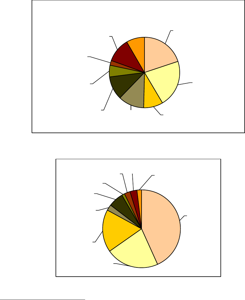
32
market requirements while maintaining the same blended average polysilicon cost (i.e., the
overall cost of contract polysilicon blended with spot polysilicon).
The Siemens process accounted for about 78% and FBR for about 16% of polysilicon produced
in 2008, with UMG-Si processes accounting for most of the rest (Barclays 2009, Mehta and
Bradford 2009, Cowen & Co. 2009, Morgan Stanley 2009, Bradford et al. 2008c). Figure 2.18
shows one analyst's estimate of 2008 production categorized by producer, and Figure 2.19 shows
it categorized by producing country (Bradford 2008).
Figure 2.18. Proportion of 2008 polysilicon production categorized by producer
(Bradford 2008)
Figure 2.19. Proportion of 2008 polysilicon production categorized by producing country
9
(Bradford 2008)
9
U.S. production includes a company with production in both the United States and Italy.
Hemlock (U.S.)
20%
Wacker
(Germany)
22%
Tokuyama
(Japan)
9%
MEMC
(U.S./Italy)
12%
REC (U.S.)
11%
Mitsubishi
(Japan)
5%
Sumitomo
(Japan)
2%
New Entrants -
Current
Technology
(Siemens/FBR)
11%
New Entrants -
Alternative
Technology
(e.g., UMG-Si)
8%
United
States
43%
Germany
22%
Japan
18%
South
Korea
3%
China
6%
Russia
1%
Norway
2%
Brazil
3%
Canada
2%
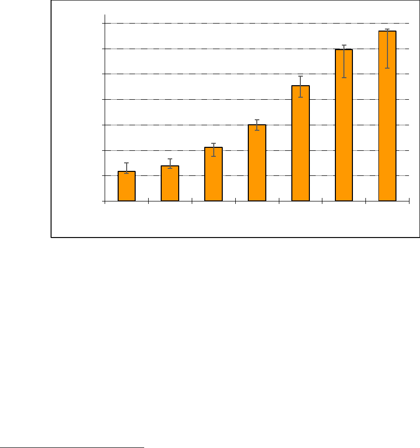
33
The global economic crisis that became apparent in late 2008, and which is expected to diminish
funds available for investments and the demand for PV, caused analysts to reduce their
projections for the growth of PV and polysilicon production (Bartlett et al. 2009). Nevertheless, a
number of analysts who released reports in early 2009 projected 157,000–203,000 MT of
polysilicon production by 2012, a two- to threefold increase over 2008 (Figure 2.20). Projecting
beyond 2010 is more difficult than making nearer-term projections, because decisions to build
new capacity need only be made 2 years in advance and thus would not need to be made by late
2008 or early 2009 (Bradford et al. 2008c). Solar applications were projected to use 80%–90% of
polysilicon supply by 2012 (Mehta and Bradford 2009, Cowen & Co. 2009).
Figure 2.20. Polysilicon supply projections through 2012
(Bartlett et al. 2009)
10
The projected increase in polysilicon supply is expected to meet or exceed PV demand for the
next several years. Several major trends will influence polysilicon supply and demand during this
period, with potential to increase supply or decrease demand beyond current projections:
• Improved silicon utilization. The PV industry has continued to improve silicon
utilization (watts of PV per gram of polysilicon) by decreasing silicon wasted
during manufacturing, producing thinner wafers, and producing cells with higher
efficiency. One analyst projects an average 14% improvement in polysilicon
utilization from 8.7 g/W in 2008 to 7.5 g/W in 2012 (Bradford 2008). Increasing
silicon utilization decreases the amount of polysilicon required to manufacture an
equivalent amount of crystalline silicon PV.
10
Projections through 2010 reflect estimates made by six analysts (Barclays 2009, Mehta and Bradford 2009,
Cowen & Co. 2009, Morgan Stanley 2009, Oppenheimer 2009, Thomas Weisel 2009), whereas projections for 2011
include data from four analysts (Barclays 2009, Mehta and Bradford 2009, Cowen & Co. 2009, Oppenheimer 2009),
and data for 2012 are from three analysts (Barclays 2009, Mehta and Bradford 2009, Cowen & Co. 2009), obtained
from Bartlett et al. 2009.
0
30
60
90
120
150
180
210
2006
2007
2008
2009
2010
2011
2012
Total Polysilicon Production (1,000 MT)
Low
Median
High

34
• Increased use of UMG-Si. As discussed above, UMG-Si processes could offer
substantial cost and time savings over the Siemens process and FBR. Significant
venture-capital UMG-Si investments in 2008 indicated continued interest in this
approach, but concerns remain about the efficiency of PV cells made with a high
percentage of UMG-Si (Bradford et al. 2008c). If technology is developed to
enable the use of UMG-Si in blends higher than the current level of 10%,
UMG-Si could become a larger source of low-cost PV feedstock. Estimates from
several industry analysts project the market share of UMG-Si rising from about
6% in 2008 to 8%–16% in 2012 (Bartlett et al. 2009).
11
• Market penetration of thin-film PV. Thin-film PV, which requires little or no
polysilicon feedstock, has become a major competitor to crystalline silicon PV.
Projections of market share rise from about 16% in 2008 to 16%–34% in 2012
(Bartlett et al. 2009).
12
Increased use of thin-film PV reduces demand for
crystalline silicon PV and polysilicon feedstock.
Other factors that could affect the supply of or demand for polysilicon include larger-than-
expected polysilicon production by companies based in China, technological breakthroughs (e.g.,
rapid penetration of concentrating PV), manufacturing disruptions (e.g., an accident in a very
large polysilicon manufacturing facility), PV supply-chain disruptions (e.g., shortages of solar-
grade graphite or glass), changes in PV-related government policies, and other "macro shocks"
(e.g., large-scale natural disasters or epidemics) (Rogol et al. 2008).
As a result of the aforementioned trends toward increased polysilicon supply and/or moderated
demand, polysilicon prices are expected to decrease over the next several years (Figure 2.21). PV
cell manufacturers may be able to minimize/stabilize the price they pay for polysilicon by
measures such as securing fixed-price contracts, producing their own polysilicon, or partnering
with polysilicon producers.
11
Barclays 2009, Mehta and Bradford 2009, Cowen & Co. 2009, Morgan Stanley 2009, as obtained from Bartlett et
al. 2009.
12
Mehta and Bradford 2009, Citi Investment Research 2009, Cowen & Co. 2009, Deutsche Bank 2009, Morgan
Stanley 2009, Navigant 2009, New Energy Finance 2009, Thomas Weisel 2009, as obtained from Bartlett et al.
2009.
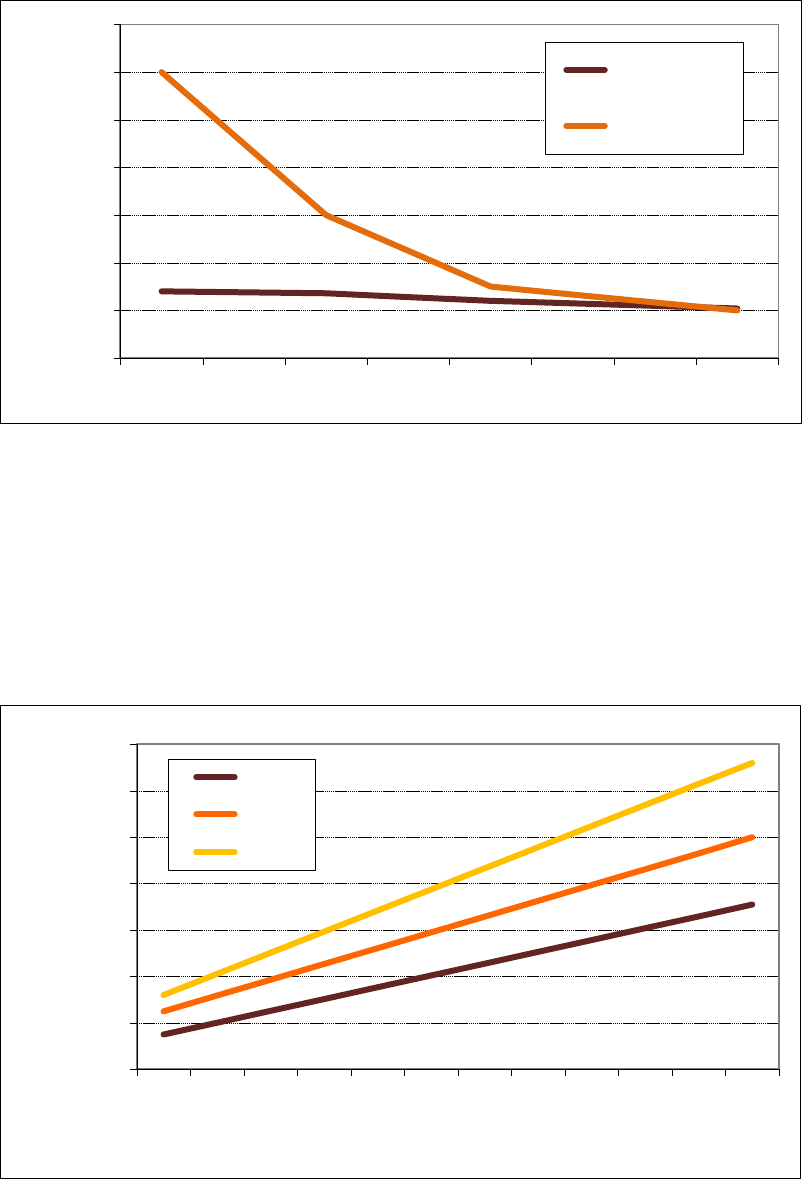
35
Figure 2.21. Polysilicon price projections through 2015
(Mehta and Bradford 2009)
Polysilicon price and silicon utilization have a substantial effect on PV module manufacturing
cost. Figure 2.22 plots module manufacturing cost (for a European-produced, multicrystalline
silicon module manufactured in 2008) versus blended polysilicon price (a weighted average of
contract and spot price) for three levels of silicon utilization. This figure illustrates the
importance to PV module economics of lowering polysilicon costs and increasing silicon
utilization (Mehta and Bradford 2009).
Figure 2.22. PV module sensitivity to polysilicon price and utilization
(Mehta and Bradford 2009)
$0
$50
$100
$150
$200
$250
$300
$350
2008
2009
2010
2011
2012
2013
2014
2015
Projected Polysilicon Price ($/kg)
Contract Price
Spot Price
$1.80
$2.00
$2.20
$2.40
$2.60
$2.80
$3.00
$3.20
$40
$50
$60
$70
$80
$90
$100
$110
$120
$130
$140
$150
Module manufacturing cost ($/W)
Blended polysilicon price ($/kg)
5 g/W
7 g/W
9 g/W

36
2.4.2 Rare Metals Supply and Demand for PV
As discussed above, thin-film PV technologies, which use 100 times less silicon than
conventional crystalline cells (e.g., for a-Si PV) or use no silicon at all (e.g., for CdTe, CIGS,
and CIS PV), are projected to garner 16%–34% of the PV market by 2012. This large-scale
production has raised concerns about the supply of rare metals such as indium, gallium, and
tellurium (Grama & Bradford 2008). Indium and tellurium have been estimated to limit total
thin-film capacity to between 100 GW for CdTe (Feltrin & Freundlich 2008) and 30 TW for
CIGS/CIS (Zweibel 2005) based on different estimates of rare metal supply.
The estimated worldwide indium reserve base
13
was 16,000 MT in 2007, and annual production
was 510 MT (Grama & Bradford 2008). CIGS PV requires approximately 20 MT of indium per
GW. With projected production growth to 3.1 GW by 2012, CIGS PV will require approximately
63 MT of indium (12% of current annual production) by that year (Grama & Bradford 2008).
Competing uses for indium include LCD displays, integrated circuits, and electronic devices.
The market price for indium reached $835/kg in early 2007, but fell to $750/kg in August 2008
(Grama and Bradford 2008). Indium recycling could increase significantly, and alternative
sources could be developed, if the indium price stays high. Indium has substitutes, but they
usually lead to losses in production efficiency or product characteristics. Gallium can be used in
some applications as a substitute for indium in several alloys. In glass-coating applications,
silver-zinc oxides or tin oxides can be used. Indium phosphide can be substituted by gallium
arsenide in solar cells and in many semiconductor applications. The United States has no primary
indium or gallium production capacity, and most reserves are located in other countries.
The estimated worldwide tellurium reserve base was as high as 47,000 MT in 2007, and annual
production was 475 MT. CdTe PV requires approximately 47 MT of tellurium per GW. With
projected production growth to 1.2 GW by 2012, CdTe PV will require approximately 55 MT of
tellurium (12% of current annual production) by that year. Competing uses for tellurium include
semiconductor and electronics products and metal alloys. The tellurium required for CdTe PV
has driven a fourfold price increase in the past 5 years; the market price increased from $50/kg in
2004 to more than $225/kg in August 2008. Tellurium recycling could increase significantly, and
alternative sources could be developed (e.g., bismuth telluride), if the tellurium price stays high.
Beyond 2012, tellurium production likely will need to increase to keep pace with demand from
the solar industry (Grama and Bradford 2008).
2.4.3 Glass Supply for PV
Glass is resistant to long-term weathering, is relatively inexpensive, and has good mechanical
strength, making it an ideal encapsulation material for crystalline silicon PV as well as an
encapsulation and substrate material for most thin-film PV. The demand for solar glass is
expected to see strong growth in conjunction with growing PV demand. Yole Development
forecasts that solar glass demand will grow from 50 million m
2
today to more than 300 million
m
2
in 2015. Mark Farber, former CEO and cofounder of Evergreen Solar, notes that PV currently
13
The U.S. Geological Survey defines base reserves as that part of an identified resource that meets minimum
physical and chemical criteria related to current production practices (Grama & Bradford 2008).
37
accounts for less than 1% of the glass market, but that it could account for up to 5% by 2012
(Podewils 2008).
The glass demand for PV (as well as for CSP) is primarily for high-quality, low-iron glass. This
demand is met by both the rolled- and float-glass markets. Rolled glass is a better choice for
solar applications because it requires 80% less energy to manufacture than float glass, it can use
resources with 30% more iron to achieve the same transparency, and it is 30% less expensive to
produce. Rolled glass currently supplies 60%–70% of the PV market, and production is growing
rapidly to meet PV demand, particularly in China. However, demand for rolled glass exceeds
supply by about 1 year. Float glass, which accounts for more than 90% of the flat glass market,
will likely supply the additional PV glass demand until the rolled glass market can catch up
(Podewils 2008).
There is an increasing trend, particularly in China, toward constructing PV-dedicated glass
factories and vertically integrating glass production in the PV supply chain by building rolled-
glass factories on site, which minimizes supply-driven price volatility and transportation costs.
China's CSG Solar Glass Co. built the first factory to produce glass exclusively for the solar
industry (Podewils 2008). Once operating at full capacity, CSG could produce enough glass for
2 GW/year of PV. CSG also is vertically integrating, from polysilicon production to finished
modules, and plans to have 450 MW of cell and module production by 2010.
2.4.4 Material and Water Constraints for CSP
Concentrating solar power facilities are constructed primarily of concrete, steel, and glass.
Although these materials are not subject to rigid supply limits, they are affected by changes in
commodity prices.
In CSP systems, steel is a commodity that cannot be substituted, and its cost rose substantially
from 2006 through the first half of 2008. These near-term price increases inflated the levelized
cost of energy (LCOE) that project developers could offer to utilities. However, the economic
downturn in the second half of 2008 brought commodities closer to pre-2006 prices (Yahoo
Finance 2009). For CSP projects to be economically viable, it will be important for steel prices to
remain at reasonable costs, as project developers do not have pricing power on this commodity
and must therefore accept the price being offered (Bullard et al 2008).
The combination of a limited number of companies producing the main CSP system components
on a commercial scale and a large construction pipeline could create a component supply
bottleneck, depending on the growth of demand. This is especially true for turbines, which
require a 24–30 month advance order by the project developer (Merrill Lynch 2008).
Conversely, several of the main materials and equipment relied on by the CSP industry could
leverage other manufacturing industries (e.g., automotive and buildings), potentially facilitating a
relatively fast production ramp-up (Andraka 2008). In addition, some companies are entering
multiple levels of the value chain, thus becoming less dependent on other companies for meeting
large supply requests (e.g., Solel and Abengoa are entering the reflector market). For these
reasons, many believe that reflector and receiver demand will not create bottlenecks in the near
future (Bullard et al. 2008, Merrill Lynch 2008).

38
Aside from the aforementioned solid materials, the availability of water resources might limit the
amount of CSP deployed in arid regions. As with fossil and nuclear power plants, the most
common and economical method for cooling a CSP plant is evaporative water cooling. A typical
parabolic trough plant requires 800 gallons of water per MWh, which can be reduced to about
80 gallons per MWh by implementing dry cooling. Dry cooling, however, requires higher capital
expenditure and is likely to decrease plant efficiency, especially under higher-temperature
conditions. The loss of efficiency is greatest for systems requiring lower operating temperatures.
Another cooling solution is to use hybrid wet/dry cooling, which uses less water than 100% wet
cooling, and also reduces efficiency losses associated with dry cooling. For closed-cycle CSP
heat engines such as dish-engine generators, air cooling is sufficient (U.S. DOE 2009).
2.4.5 Land and Transmission Constraints for Utility-Scale Solar
Solar project developers have been attracted to numerous locations in the Southwest, evident
from a surge of more than 220 applications received by the U.S. Bureau of Land Management
for new solar power plants (Resseguie 2008). However, transmission in many of these areas is
lacking and substantial upgrades to the western grid will be necessary for projects to move
forward. Moreover, land-use conflicts exist, as a large percentage of the area is federal land
traditionally set aside for conservation and recreational purposes. To address the transmission,
grid upgrade, and land-use issues, a number of major multi-agency agreements and initiatives
have arisen at the national, state, and regional levels. Five such agreements and initiatives are
described in this section.
The U.S. Bureau of Land Management (BLM) and DOE are collaborating on a Solar
Programmatic Environmental Impact Statement (PEIS). The PEIS will identify the impacts of,
and develop better management strategies for, utility-scale solar development on the public lands
of six states (Arizona, California, Colorado, New Mexico, Nevada, and Utah). The BLM has
announced the availability of maps that identify 24 tracts of BLM-administered land for in-depth
study for solar development and requested public comment on those study areas; the schedule for
release of the draft PEIS will be determined after the evaluation of those comments. Further
details can be found at http://solareis.anl.gov
, and solar energy study area maps are available at
http://solareis.anl.gov/eis/maps/index.cfm.
The Western Governors’ Association (WGA) and DOE launched the Western Renewable Energy
Zones (WREZ) Project in May 2008. WREZ involves working groups that are identifying high-
resource areas to include in energy development and environmentally sensitive lands to exclude
from this development. The assessment was presented to the WGA for approval in June 2009,
concluding phase one of the process. Subsequent phases will develop a modeling tool and a high-
level transmission plan coordinated through the Western Electricity Coordinating Council. More
information is available at http://www.westgov.org/.
Most recently, a multi-agency memorandum of understanding (MOU) was signed in October
2009 regarding coordination in federal agency review of electric transmission facilities on
federal land. The MOU was signed by the U.S. Department of the Interior, Department of
Agriculture, Department of Commerce, Department of Defense, Department of Energy,
Environmental Protection Agency, Council on Environmental Quality, Federal Energy
Regulatory Commission (FERC), and the Advisory Council on Historic Preservation. The

39
agreement supersedes an earlier MOU signed in August 2006. The October 2009 MOU will cut
approval time off the normal federal permit process and help break down the barriers to siting
new transmission lines by: 1) designating a single federal point-of-contact for all federal
authorizations; 2) facilitating coordination and unified environmental documentation among
project applicants, federal agencies, states, and tribes involved in the siting and permitting
process; 3) establishing clear timelines for agency review and coordination; and 4) establishing a
single consolidated environmental review and administrative record (U.S. DOI 2009).
In California, the Renewable Energy Transmission Initiative (RETI) is a collaboration of public
and private entities whose objective is to provide information to policymakers and stakeholders
on the transmission requirements to access cost-effective, environmentally sensitive, renewable
energy resources. Phase one of the initiative, completed at the start of 2009, identified and
ranked zones in California and nearby states that can provide and competitively deliver
renewable energy to the state. Phase two, which includes developing conceptual transmission
plans and refining previous work, is under way. Additional information is available at
www.energy.ca.gov/reti.
Another development in California was an MOU signed in August 2007 between the U.S.
Bureau of Land Management (BLM) (part of the U.S. Department of the Interior) and the
California Energy Commission (CEC) to document the roles, responsibilities, and procedures to
follow in conducting a joint environmental review of proposed solar thermal power plant
projects in the state of California. A number of these projects are proposed to be built in
California on land owned by the federal government and managed by BLM. Because projects
need both a right-of-way from BLM and certification from CEC, coordination in the preparation
of an environmental analysis for each of these projects will avoid duplication of efforts, promote
intergovernmental coordination at the federal, state, and local levels, and facilitate public review
by providing a joint document and a more efficient review process (CEC 2007a).
The long approval process for a recent transmission project in California provides an example of
a project that could have benefited from the type of coordination being carried out through the
above agreements and initiatives. After 3 years and several major revisions, the 1-GW, 123-mile
Sunrise Powerlink Transmission Project was approved by the California Public Utilities
Commission in December 2008. This project allows San Diego Gas & Electric to connect
producers in the Imperial Valley of California to end users in the San Diego area, and is expected
to be completed in 2012. The process for obtaining the permit was arduous because of the initial
lack of disclosure by the proponent, the environmental sensitivity of the land proposed to be
developed, and the number of stakeholders involved (Herndon 2009). Many PV and CSP
projects in the planning stages are dependent on the construction of this line.
2.5 Solar Industry Employment Trends
Because of the rapid expansion of the solar industry over the past several years, employers are
reporting increasing difficulty in finding qualified people to hire. As a result, labor supply and
demand within the solar industry, and the manner in which the two are tied to educational and
training opportunities, has recently become a topic of strong interest to both industry and
government. The possibility of labor shortages within the industry and a surge of interest in

40
green jobs as a contributor to economic recovery are two factors driving state and federal
initiatives. If Germany is any indication of how fast the U.S. solar industry can grow without
experiencing major bottlenecks in labor supply, then it is possible that the U.S. educational and
training infrastructure could meet the needs of the industry over the next several years.
Despite the poor investment climate that is clouding economic growth in the United States and
abroad, the extension and enhancement of the federal investment tax credit (ITC) as of October
2008 and additional policy enhancements and economic incentives resulting from the American
Recovery and Reinvestment Act (ARRA) in February 2009 are expected to encourage industry
expansion and job creation. In particular, the elimination of the residential investment tax credit
cap (effective January 2009) should result in more business for PV system installers. Also, the
new ability of utilities to take advantage of the ITC could result in very large installations being
constructed and could help lead to the establishment of well-defined career pathways for PV
system designers and solar electricians. For more details on recent federal policy developments
that may encourage job growth in the solar industry, see Section 4.1 of this report.
Though not the focus of this section, studies have quantified the job creation potential of
renewable energy as compared to fossil fuel technologies. A recent study by analysts at U.C.
Berkeley concluded that renewable energy technologies generate more jobs per unit of energy
than fossil fuel-based technologies. Among the renewable energy technologies, solar PV creates
the most jobs per unit of electricity output. Solar PV was estimated to create 0.87 job-
years/GWh, whereas natural gas and coal were each estimated to create 0.11 job-years/GWh.
Solar PV thus generates almost eight times as many job-years/GWh as natural gas or coal (Wei
et al. 2010).
14
2.5.1 Types of Jobs in the PV and CSP Industries
The following are examples of occupations associated with the manufacture and installation of
PV and CSP.
• Manufacturing positions include factory worker, sheet metal worker, glass worker,
technician (e.g., semiconductor for PV), material handler, factory supervisor,
manufacturing manager, engineer (quality assurance, manufacturing, chemical process,
mechanical, electrical, optical), material scientist.
• Installation positions include solar system installer/technician (PV), solar system designer
(PV), technical sales representative and estimator (PV), architect (PV), roofing contractor
(PV), general contractor, supervisor/foreman, heavy construction worker, welder,
pipefitter, engineer (mechanical, electrical, civil).
• Administrative and support positions include administrative assistant, purchasing agent,
accountant, health and safety officer, information technology professional, director.
Jobs in the solar industry fall into three categories: direct, indirect, or induced. Direct jobs are
those within the solar industry (e.g., manufacturing, installation, R&D); indirect jobs are those in
industries that support the solar industry (e.g., jobs in the polysilicon, glass, and steel industries);
and induced jobs are those that result from the economic activity stimulated by the solar industry
14
See http://rael.berkeley.edu/greenjobs for more details.

41
(e.g., people buying more goods and services in a region where there is a new PV manufacturing
plant or where a new PV or CSP installation is under construction).
Estimating numbers of jobs is a challenging task that is generally performed by surveying
employers and industry analysts or by using economic input-output models that account for jobs
based on the trail of goods and services leading up to, and after, production. There is significant
variation in job number and labor intensity estimates, which results from many factors,
including:
• Data collection and analysis method
• Types of jobs being considered (e.g., direct, indirect, and induced)
• Types of occupations being considered (e.g., factory worker, installer, salesperson).
• Variation in estimates of capacity being installed (for job forecasts)
• Technologies included (e.g., PV, CSP, solar water heating)
• Types of industry subsectors included (residential new and retrofit, commercial, utility,
remote or off-grid)
• Variation in metrics or units being used
• Variation in the time periods being considered, such as the lifespan of an installation or
within only a certain phase (e.g., construction, O&M)
• Whether a study is measuring gross or net job impacts (net impacts account for
displacement of jobs in other industries such as coal or natural gas).
In this and many reports, the unit of measure used for jobs is the job-year or full-time equivalent
(FTE), which represents full-time employment for one person for the duration of a year. A
common metric for labor intensity is jobs/MW (or FTEs/MW), although other metrics such as
jobs per MWh or jobs per dollar invested are also used depending on the question of interest.
2.5.2 Current and Projected Employment in the Solar Industry, Global and U.S.
In 2008, an estimated 173,000 people
15
were employed worldwide in the solar electric industry,
according to a 2009 New Energy Finance (NEF) study (McCrone et al. 2009). Most of these jobs
were in the PV manufacturing value chain and in the construction and installation of PV
components and projects.
16
Of the 173,000 jobs, the PV industry contributed about 169,000 and
the CSP industry about 4,000. The 169,000 PV jobs correspond to 5.8 GW produced and
installed globally in 2008 and 14.7 GW of cumulative installed PV capacity through 2008.
17
An earlier report produced by the United Nations Environment Programme (UNEP) in 2008
compiled an estimate of global PV employment based on five industry leaders: Germany, Spain,
China, Japan, and the United States. PV jobs in these countries together amounted to
approximately 170,000 jobs
18
15
These are direct and indirect jobs, in FTEs. The figure includes jobs in PV and CSP for electricity generation, not
solar hot water heating jobs. Also not included are induced jobs.
worldwide in 2007 (Renner et al. 2008). The 170,000 job number
16
All job and labor intensity figures quoted in this section from the McCrone et al., New Energy Finance article of
2009 refer to FTEs.
17
The 14.7 GW of cumulative installed PV capacity through 2008 is higher than the 13.9-GW estimate provided in
Section 1.1.1 of this report. Estimates of cumulative installed PV capacity through 2008 range from 13-17 GW.
18
The figure of 170,000 total jobs worldwide provided in the UNEP report includes direct and indirect jobs.

42
for 2007 is similar to the NEF number of 169,000 PV jobs in 2008 (though the estimates are one
year apart). However, as previously stated, it is not unusual for job estimates to vary based on
many factors, including differences in methodology and metrics, which jobs in the value chain
are being counted, and in this case, for which year and which countries the data are being
provided.
Of the 170,000 global PV jobs reported by UNEP for the year 2007, China held the most jobs,
with 70% of its 55,000 jobs going to the manufacture of PV cells, modules, and processed
silicon. Germany
19
Estimates of U.S. PV jobs for the year 2007 range from 6,000 to 20,000 jobs. EIA reports
employment in the PV manufacturing industry to be about 6,200 jobs in 2007, based on a survey
of PV cell/module manufacturers (EIA 2008a). The EIA number does not include all jobs along
the PV value chain and does not include indirect jobs. By comparison, for the year 2007, ASES
reported 8,700 direct jobs and 19,800 direct plus indirect jobs (ASES and MISI 2008). For the
year 2008, EIA’s survey yielded about 11,250 jobs in PV cell/module manufacturing (EIA
2009). If one used the EIA 2007 and 2008 numbers as an estimate for direct PV jobs, and used a
multiplier of 1.4 indirect jobs for every direct job, then direct plus indirect PV jobs for 2007 and
2008 would be about 14,800 and 27,000 jobs, respectively.
and Spain held approximately 35,000 and 26,000 jobs, respectively, in 2007.
Japan’s PV employment levels were estimated to be similar to Germany’s (Renner et al. 2008).
U.S. PV jobs reported by UNEP were 6,800 direct and 15,700 direct plus indirect jobs for the
year 2006, based on an estimate provided by ASES (Bezdek 2007). However, there is a large
range in the estimates of U.S. PV jobs provided by various studies.
20
Regarding projected employment in the United States, Navigant Consulting published an
employment impact study in September 2008 based on the assumption that the federal
investment tax credit (ITC) would be extended. A month later, the Emergency Economic
Stabilization Act (EESA) of 2008 extended and enhanced the ITC (beyond the assumptions
made in the Navigant study). The Navigant study estimated that 440,000 jobs
21
would be created
in the U.S. solar industry in 2016 if the ITC were extended for 8 years, which is 276,000 more
jobs than would have been created with only a reduced ITC (the residential ITC expiring and the
commercial ITC reduced to 10% at the end of 2008).
22
Of the 440,000 projected jobs in 2016,
110,000 were estimated to be direct, 130,000 indirect, and 200,000 induced (Navigant
Consulting 2008). The breakout by technology is 377,000 PV jobs, 38,000 CSP jobs, and 24,000
solar water heating jobs. The study methodology involved using economic multipliers to
calculate indirect and induced jobs from direct jobs; the multipliers are different for construction
and manufacturing versus O&M jobs (Navigant Consulting 2008, Grover 2007).
23
19
In Germany in 2008, total renewable energy jobs were about 278,000, with direct plus indirect solar industry jobs
at 74,400 or 27% of the total, and about 51,000 of solar jobs attributable to PV (the rest to solar thermal heating)
(Böhme et al. 2009). The increase from 35,000 jobs in 2007 to 51,000 in 2008 reflects 46% employment growth.
20
Job multipliers are described further in the subsequent discussion of the Navigant employment impact study.
21
Includes direct, indirect, and induced FTEs for PV, CSP, and solar water heating.
22
The 440,000 total jobs corresponds to nearly 6.5 GW of solar installations added in 2008 and 28 GW of
cumulative solar installations through 2008 in the extended ITC scenario. By comparison, the reduced ITC scenario
resulted in 9 GW of cumulative installed capacity through 2008, 19 GW less than the extended ITC scenario.
23
For construction and manufacturing, the ratio of indirect to direct is 1.4, and induced to direct is 2.1. For O&M,
the ratios are 0.5 for indirect to direct and 0.8 for induced to direct.

43
2.5.3 Labor Intensity in the PV Industry, Global and U.S.
Total employment in the solar industry is projected to increase over the next 8 years, but labor
intensity could decrease over time resulting from increased automation, economies of scale, and
greater efficiencies in the use of labor throughout the supply chain. Employment at the point of
installation is a significant component of labor intensity, thus benefiting local economies.
As with estimates of job numbers, labor intensity estimates for PV vary widely, with a range of
25 jobs/MW to more than 50 jobs/MW (including direct and indirect jobs). As discussed earlier,
the wide range is due to many factors including differences in methodology, which jobs along
the value chain are being counted, and the types of indirect jobs considered.
A recent study by New Energy Finance estimated global PV labor intensity in 2008 to be just
over 28 jobs/MW, including direct and indirect FTEs (McCrone et al. 2009).
24
The components
of the 28 jobs/MW along the value chain are presented in Table 2.3. PV operation/maintenance
(O&M), project construction, and rooftop installation accounted for 43% of PV jobs in 2008
(O&M by itself was 5%). Manufacture of silicon, wafers, cells, and modules accounted for 50%
of PV jobs in 2008. Adding induced jobs to the PV labor intensity of 28 jobs/MW using the
multipliers provided in section 2.5.2 (see footnotes) amounts to nearly 53 jobs/MW.
25
Table 2.3. Global PV Labor Intensity in 2008 (Direct and Indirect Jobs)
Job Category GW Jobs/MW Total Jobs
Operation
14.7
0.6
8,820
PV project construction and
rooftop installation
26
5.8
11 63,800
Silicon and wafers
5.8
3.5
20,300
Cell manufacture
5.8
5
29,000
Module manufacture
5.8
6
34,800
Inverters
5.8
1.3
7,540
Research
5.8
0.4
2,320
Development and services
5.8
0.4
2,320
Total
28.2
168,900
McCrone et al. 2009
The 28 jobs/MW worldwide labor-intensity number for 2008 is projected to decrease to about
13 jobs/MW in 2025 (McCrone et al. 2009). The labor-intensity estimate for 2025 is based on
24
A highly referenced labor-intensity figure for the U.S. PV industry has been 35.5 jobs/MW installed, which
originates from a study conducted by the Renewable Energy Policy Project (REPP) in 2001.
24
The study focused on
jobs along the value chain that are required to create a 2-kW residential PV system, and therefore does not factor in
commercial or utility-scale systems. The 35.5 job/MW figure includes mostly direct plus some indirect jobs.
25
Let x = direct jobs. Using the construction and manufacturing multipliers for the sake of simplicity, direct +
indirect jobs = x + 1.4x = 2.4x = 28.2. So x = 28.2/2.4 or 11.75 jobs. Total jobs = x + 1.4x + 2.1x = 4.5x =
4.5(11.75) = 52.875 or about 53 jobs. In summary: the multiplier for total to direct jobs is 4.5, the multiplier for total
jobs given direct + indirect jobs is 1.875, and the multiplier for induced jobs given direct + indirect jobs is 0.875.
26
The PV project construction and rooftop installation components were combined based on the data in the New
Energy Finance report for the purpose of presenting a global labor intensity for all PV system types.

44
39 GW of PV production and installation and 340 GW of cumulative installed PV capacity in
2025. The share of PV jobs in 2025 attributed to O&M increases to 29% (compared to 5% in
2008) based on the large cumulative installed PV capacity. PV project construction and rooftop
installation account for 33%, whereas manufacture of silicon and wafers, cell, and modules
account for 27% of PV jobs in 2025. Wafer, cell, and module manufacturing, system integration,
and residential installations are projected to have the most dramatic drops in labor intensity,
whereas commercial and utility installations will see only a slight decrease, one cause being that
many of the efficiencies in these areas have already been realized (Navigant Consulting 2008).
NREL discussions with several U.S. PV installation companies in 2008 also confirmed a pattern
of decreasing labor intensity. In addition, other insights from these conversations included the
following:
• Most installation companies do not have well-defined business groups targeting
residential, commercial, and utility markets.
• Many installation companies anticipate substantial growth in the retrofit residential
market.
• The retrofit market seems to need more skilled sales people as growth continues.
• Smaller companies are using skilled employees to do some unskilled work.
2.5.4 Employment and Labor Intensity in the U.S. and Global CSP Industry
As with PV installations, the construction phase of a CSP facility, as opposed to the operation
phase, results in the greatest economic impact. A report by NREL examining the economic
impacts of constructing a 100-MWe CSP facility in the United States, specifically Nevada,
estimated that each year of a 3-year construction period would result in slightly more than 800
direct jobs and approximately 1,600 indirect and induced jobs (Schwer and Riddel 2004).
27
This
equates to 8 direct jobs/MW and 24 jobs/MW including indirect and induced jobs, just for
construction. In addition, 0.45 jobs per MW are created directly during the operations and
maintenance phase.
28
Another U.S. example for CSP is the 400-MWe Ivanpah Solar Electric Generating System
(ISEGS) proposed for a site in California’s Mojave Desert, a power tower plant that would take
4 years to build and require approximately 500 jobs averaged over the construction period,
amounting to 1.25 jobs/MW during this time (CEC 2007b). The project also would require
100 full-time jobs for O&M, equivalent to 0.25 jobs per MW. ISEGS is a very large system, and
actually is a staged cluster of four separate CSP systems, which could explain the lower O&M
labor intensity.
By comparison, Black & Veatch estimated more than twice that number
for O&M, namely that every megawatt of CSP constructed results in 0.94 permanent O&M jobs
(Stoddard et al. 2006). It is unclear, however, whether the higher number includes indirect as
well as direct jobs.
27
The term “MWe” stands for “megawatt electrical,” and is used to distinguish electrical generation from thermal
generation at CSP plants.
28
Direct jobs are in FTEs. In total, 140 O&M jobs are created annually when including indirect and induced jobs.

45
Globally, CSP labor intensity in 2008 is estimated to be 23 jobs/MW (including direct and
indirect FTEs), which comprises the following components: operation, 0.8 jobs; project
construction, 12 jobs; manufacturing, 10 jobs; and development and services, 0.4 jobs (McCrone
et al. 2009).
2.5.5 Quality Assurance and Certification for Solar PV Installation
Proper installation of solar PV systems is essential for accelerating market acceptance and
maintaining consumer confidence. DOE SETP supports multi-tiered training and certification
processes for solar installation technicians by providing funding to the North American Board of
Certified Energy Practitioners (NABCEP), the only North American organization developing
and implementing consistent standards. Between years 2003 and 2008, NABCEP certified
587 PV installers
29
and awarded its Certificate of Basic Knowledge to 999 people.
30
2.5.6 DOE Response to Current Barriers in Workforce Development
The number
of PV installer certificates issued rose by 22% in 2008, and the number of Certificates of Basic
Knowledge awarded rose by more than 100%.
Research into workforce development tends to focus on estimating the number of jobs that will
result from enactment of regulatory policies such as state renewable portfolio standards (RPSs)
or financial incentives such as the ITC. Establishing baselines for the number of jobs within the
solar industry has proved to be difficult, and researchers often are hindered by the lack of
detailed data on occupations found in the solar industry. Based on a submission by DOE SETP,
however, the Office of Management and Budget (OMB) announced on January 21, 2009, that the
Standard Occupational Classification for 2010 will be revised to include the occupation of “Solar
Photovoltaic Installer” (47–2231), thus making it easier to track the number of PV technicians
and installers.
To better assess the education, training, and workforce development needs of the solar industry,
SETP activities in 2009 included:
• Commencing the development of the Solar Installer Instructor Training network, a multi-
year effort to provide funding to current educational providers to help train instructors at
other educational institutions that are starting training programs for the downstream PV
workforce.
• Exploring ways to provide support to activities that promote higher education in solar
technologies and upstream workforce development.
• Providing funding for research and analysis on knowledge gaps, including an
investigation of critical occupational profiles and estimates of employment within the
solar industry.
29
It is estimated that NABCEP-certified PV installers represent approximately 10% of the total number of PV
installers in the United States.
30
Professionals holding this certificate have demonstrated an understanding of the basic terms and operational
aspects of a PV system, but the certificate by itself does not qualify an individual to install PV systems. The
Certificate of Knowledge is held not only by persons interested in becoming installers, but also by industry
salespeople, contractors, local code officials, utility inspectors, and others.

46
• Through a memorandum of understanding signed in May 2009, partnering with the
Departments of Labor and Education in leveraging resources to provide green jobs
training and expertise.
• Collaborating with federal agencies and other organizations to provide more accessible
labor statistics.
2.6 References
The American Solar Energy Society (ASES) and Management Information Services, Inc. (MISI)
(2008). Defining, Estimating, and Forecasting the Renewable Energy and Energy Efficiency
Industries in the U.S. and in Colorado.
http://www.ases.org/index.php?option=com_content&view=article&id=465&Itemid=58.
Accessed December 2009.
Andraka, C.E. (July 2, 2008). Statement of Charles E. Andraka, Sandia National Laboratories.
Concentrating Solar Power. United States Senate Committee on Energy and Natural Resources
Field Hearing in Albuquerque, New Mexico.
Barclays. (2009). Solar Energy Handbook: The Second Growth Phase of Solar Era. Barclays
Capital.
Bartlett, J.E.; Margolis, R.M.; Jennings, C.E. (2009). The Effects of the Financial Crisis on
Photovoltaics: An Analysis of Changes in Market Forecasts from 2008 to 2009. National
Renewable Energy Laboratory. NREL Report no. TP-6A2-46713.
Bezdek, B. (2007). Renewable Energy and Energy Efficiency: Economic Drivers for the 21
st
Century. Boulder, CO: American Solar Energy Society.
http://www.ases.org/index.php?option=com_content&view=article&id=465&Itemid=58.
Accessed November 2009.
Böhme, D.; Dürrschmidt, W.; Van Mark, M., eds. (June 2009). Renewable Energy Sources in
Figures: National and international development. Berlin, Germany: Federal Ministry for the
Environment, Nature Conservation and Nuclear Safety (BMU).
http://www.erneuerbare-
energien.de/inhalt/5996/3860/. Accessed November 20, 2009.
Bradford, T. (2008). Polysilicon: Supply, Demand, and Implications for the PV Industry.
Prometheus Institute and Greentech Media.
Bradford, T.; Letendre, S.; Flynn, H.; Maycock, P. (March 2006). “22nd Annual Data
Collection.” PV News. Prometheus Institute and Greentech Media.
Bradford, T.; Englander, D.; Lewin, A.; Maycock, P. (2008a). March 2008. “24th Annual Data
Collection - Preliminary.” PV News. Prometheus Institute and Greentech Media.
Bradford, T.; Englander, D.; Lewin, A.; Maycock, P. (2008b). April 2008. PV News. “Letter
from the Editor.” Prometheus Institute and Greentech Media.
Bradford, T.; Englander, D.; Lewin, A.; Maycock, P. (2008c). May 2008. PV News. “Polysilicon
Forecasts through 2012.” Prometheus Institute and Greentech Media.

47
Bradford, T.; Englander, D.; Smith, F.; Maycock, P. (April 2009). “25th Annual Data Collection
Results: PV Production Explodes in 2008.” PV News. Prometheus Institute and Greentech
Media.
Bullard, N.; Chase. J.; d’Avack, F. (May 20, 2008). “The STEG Revolution Revisited.” Research
Note. London: New Energy Finance.
California Energy Commission (CEC). (2007a). August 2007. “Memorandum of Understanding
Between the U.S. Department of the Interior, Bureau of Land Management California Desert
District, and the California Energy Commission Staff Concerning Joint Environmental Review
for Solar Thermal Power Plant Projects.”
http://www.energy.ca.gov/siting/solar/BLM_CEC_MOU.PDF. Accessed November 23, 2009.
California Energy Commission (CEC). (2007b). October 12, 2007. Ivanpah Application for
Certification, Executive Summary.
http://www.energy.ca.gov/sitingcases/ivanpah/documents/applicant/AFC/Volume1/. Accessed
November 23, 2009.
Citi Investment Research. (2009). U.S. Solar Stocks: Inventory Has Yet to Peak, so It’s Still Too
Early. Citi Investment Research.
Cowen & Co. (2009). Industry Outlook: Industry Hoping for Help from Stimulus Bill. Cowen &
Co.
Deutsche Bank. (2009). Solar Photovoltaic Industry: Looking Through the Storm. Deutsche
Bank.
Emerging Energy Research. (2007). Global Concentrated Solar Power Markets and Strategies,
2007–2020. Cambridge, MA: Emerging Energy Research.
Feltrin, A.; Freundlich, A. (2008). “Material Considerations for Terawatt Level Deployment of
Photovoltaics.” Renewable Energy, 33, pp.180–185.
First Solar Inc. (2008). “Corporate Overview Q3 2008.” First Solar Web site.
http://investor.firstsolar.com/phoenix.zhtml?c=201491&p=irol-irhome. Accessed March 17,
2009.
Grama, S.; Bradford, T. (2008). Thin-Film PV 2.0: Market Outlook Through 2012. Prometheus
Institute and Greentech Media.
Grama, S.; Wayman, E.; Bradford, T. (2008) Concentrating Solar Power—Technology, Cost,
and Markets. 2008 Industry Report. Cambridge, MA: Prometheus Institute and Greentech
Media.
Grover, S. (2007). Energy, Economic, and Environmental Benefits of the Solar America
Initiative. Prepared for the National Renewable Energy Laboratory by ECONorthwest. NREL
Report SR-640-41998.
Herndon, A. (January 20, 2009). “Sunrise in the West: California’s $1.9bn Renewable Energy
Transmission Line.” Analyst Reaction. London: New Energy Finance.
Maycock, Paul D. (February 2002). “World PV Cell/Module Production (1988-2001).” PV
News.

48
McCrone, A.; Peyvan, M.; Zindler, E. (June 17, 2009). “Net Job Creation to 2025: Spectacular in
solar, but modest in wind.” Research Note. London: New Energy Finance.
Mehta, S.; Bradford, T.; (2009). PV Technology, Production, and Cost, 2009 Forecast: The
Anatomy of a Shakeout. Prometheus Institute and Greentech Media.
Merrill Lynch. (2008). Solar Thermal: Not Just Smoke and Mirrors. New York, NY: Merrill
Lynch.
Morgan Stanley. (2009). Solar Devices: Dislocation – Industry Reset. Morgan Stanley.
Mints, P.; Tomlinson, D. (2007). Photovoltaic Manufacturer Shipments & Competitive Analysis
2006/2007. Report # NPS-Supply2. Palo Alto, CA: Navigant Consulting Photovoltaic Service
Program.
Mints, P.; Tomlinson, D. (2008). Photovoltaic Manufacturer Shipments & Competitive Analysis
2007/2008. Report # NPS-Supply3. Palo Alto, CA: Navigant Consulting Photovoltaic Service
Program.
Mints, P. (2009). Photovoltaic Manufacturer Shipments, Capacity, & Competitive Analysis
2008/2009. Report # NPS-Supply4. Palo Alto, CA: Navigant Consulting Photovoltaic Service
Program.
Navigant Consulting (2008). Economic Impacts of Extending Federal Solar Tax Credits.
Prepared for the Solar Energy Research and Education Foundation (SEREF).
http://www.seia.org/cs/news_research_and_multimedia/research/. Accessed February 2009.
Oppenheimer. (2009). PV Market Forecast. Oppenheimer & Co.
Podewils, C. (February 2008). “On the glass path.” Photon International. pp.74–79.
Renner, M.; Sweeney, S.; Kubit, J. (2008). Green Jobs: Towards decent work in a sustainable,
low-carbon world. Washington, DC: Worldwatch Institute. Commissioned and funded by United
Nations Environment Programme (UNEP).
http://www.unep.org/labour_environment/features/greenjobs-report.asp. Accessed July 2009.
Resseguie, L. (November 2008). E-mail correspondence. U.S. Bureau of Land Management
(BLM).
Rogol, M.; Choi, P.; Conkling, J.; Fotopoulos, A.; Peltzman, K.; Roberts, S. (2006). Solar
Annual 2006: The Gun Has Gone Off. Solar Verlag GmbH/Photon Consulting.
Rogol, M.; Farber, M.; Flynn, H.; Meyers, M.; Paap, S.; Porter, C.; Rogol, J.; Song, J. (2008).
Solar Annual 2008: Four Peaks. Photon Consulting.
Schwer, R.K.; Riddel, M. (February 2004). The Potential Economic Impact of Constructing and
Operating Solar Power Generation Facilities in Nevada. Prepared for the National Renewable
Energy Laboratory by the Center for Business and Economic Research at UNLV. NREL Report
SR-550-35037.
Stoddard, L.; Abiecunas, J.; O’Connell, R. (April 2006). Economic, Energy and Environmental
Benefits of Concentrating Solar Power in California. Prepared for the National Renewable
Energy Laboratory by Black & Veatch. NREL Report SR-550-39291.
Thomas Weisel. 2009. Alternative Energy; Presentation Materials to Investors. Thomas Weisel
Partners.

49
U.S. DOE. (2009). Report to Congress. Concentrating Solar Power Commercial Application
Study: Reducing Water Consumption of Concentrating Solar Power Electricity Generation. U.S.
Department of Energy, www.eere.energy.gov/solar/pdfs/csp_water_study.pdf.
U.S. Department of Energy, Energy Information Administration (EIA). (2008a). Solar
Photovoltaic Cell/Module Manufacturing Activities 2003-2007.
http://www.eia.doe.gov/cneaf/solar.renewables/page/solarreport/solarpv.html. Accessed May 28,
2009.
U.S. Department of Energy, Energy Information Administration (EIA). (2008b). Solar Thermal
and Photovoltaic Collector Manufacturing Activities 2003-2007.
http://www.eia.doe.gov/cneaf/solar.renewables/page/solarreport/solar.html. Accessed May 28,
2009.
U.S. Department of Energy, Energy Information Administration (EIA). (2009). Solar
Photovoltaic Cell/Module Manufacturing Activities 2008.
http://www.eia.doe.gov/cneaf/solar.renewables/page/solarreport/solarpv.pdf. Accessed January
12, 2010.
U.S. Department of the Interior (DOI). October 28, 2009. “Memorandum of Understanding
among the U.S. Department of Agriculture, Department of Commerce, Department of Defense,
Department of Energy, Environmental Protection Agency, the Council on Environmental
Quality, the Federal Energy Regulatory Commission, the Advisory Council on Historic
Preservation, and the Department of the Interior, regarding coordination in federal agency review
of electric transmission facilities on federal land.”
http://www.doi.gov/news/09_News_Releases/102809a.html. Accessed November 25, 2009.
Wei, M; Patadia, S.; Kammen, D. (2010). “Putting Renewables and Energy Efficiency to Work:
How Many Jobs Can the Clean Energy Industry Generate in the U.S.?” Energy Policy. Volume
38. pp. 919-931. http://rael.berkeley.edu/greenjobs. Accessed January 12, 2010.
Winegarner, R.M.; Johnson, R.O. (2006). Polysilicon 2006. Sage Concepts, Inc./Solar Insights
LLC.
Wu, J.; Chase, J. (2009). “Silicon and Wafer Spot Price Index.” Analyst Reaction. London: New
Energy Finance.
Yahoo Finance. (2009). Market Vectors Steel ETF (SLX).
http://finance.yahoo.com/q/hp?s=SLX&a=11&b=31&c=2005&d=00&e=1&f=2009&g=m.
Accessed July 2009.
Zweibel, K. (2005). The Terawatt Challenge for Thin-Film PV. NREL/TP-520-38350. Golden,
CO: National Renewable Energy Laboratory.
50
3. Cost, Price, and Performance Trends
This chapter covers cost, price, and performance trends for PV and CSP. Sections 3.1 and 3.2
discuss levelized cost of energy, solar resource, and capacity factor for PV and CSP. Section 3.3
provides information on efficiency trends for PV cells, modules, and systems. Section 3.4
discusses PV module reliability. Sections 3.5 and 3.6 cover PV module and installed-system cost
trends. Section 3.7 discusses PV operations and maintenance (O&M) trends. Section 3.8
summarizes CSP installation and O&M cost trends, and Section 3.9 presents information on the
characteristics and performance of various CSP technologies.
3.1. Levelized Cost of Energy, PV and CSP
Levelized cost of energy (LCOE) is the ratio of an electricity-generation system's amortized
lifetime costs (installed cost plus lifetime O&M costs) to the system's lifetime electricity
generation. The calculation of LCOE is highly sensitive to installed system cost, O&M costs,
location, orientation, financing, and policy. Thus it is not surprising that estimates of LCOE vary
widely across sources.
One recent source estimates that worldwide, the range of LCOE is approximately $0.20–$0.80
per kWh for rooftop PV and $0.12–$0.18 per kWh for parabolic trough CSP, not including
government incentives (REN21 2008). The wide LCOE range for PV ($0.20–$0.80 per kWh) is
due largely to the effect on LCOE of location and the corresponding solar radiation (insolation).
Worldwide, typical PV LCOE ranges are $0.20–$0.40 per kWh for low latitudes with high
insolation of 2,500 kWh/m
2
/year, $0.30–$0.50 per kWh for 1,500 kWh/m
2
/year (typical of
Southern Europe), and $0.50–$0.80 per kWh for 1,000 kWh/m
2
/year (higher latitudes) (REN21
2008). See Figure 3.2 for a map of the solar resource in the United States, Germany, and Spain.
Figure 3.1 shows LCOE for residential PV systems in selected U.S. cities ranging from about
$0.20/kWh to more than $0.32/kWh (when calculated with the federal ITC) based on the quality
of the solar resource. Without the ITC, the range for these same cities is about $0.28/kWh to
$0.46/kWh.
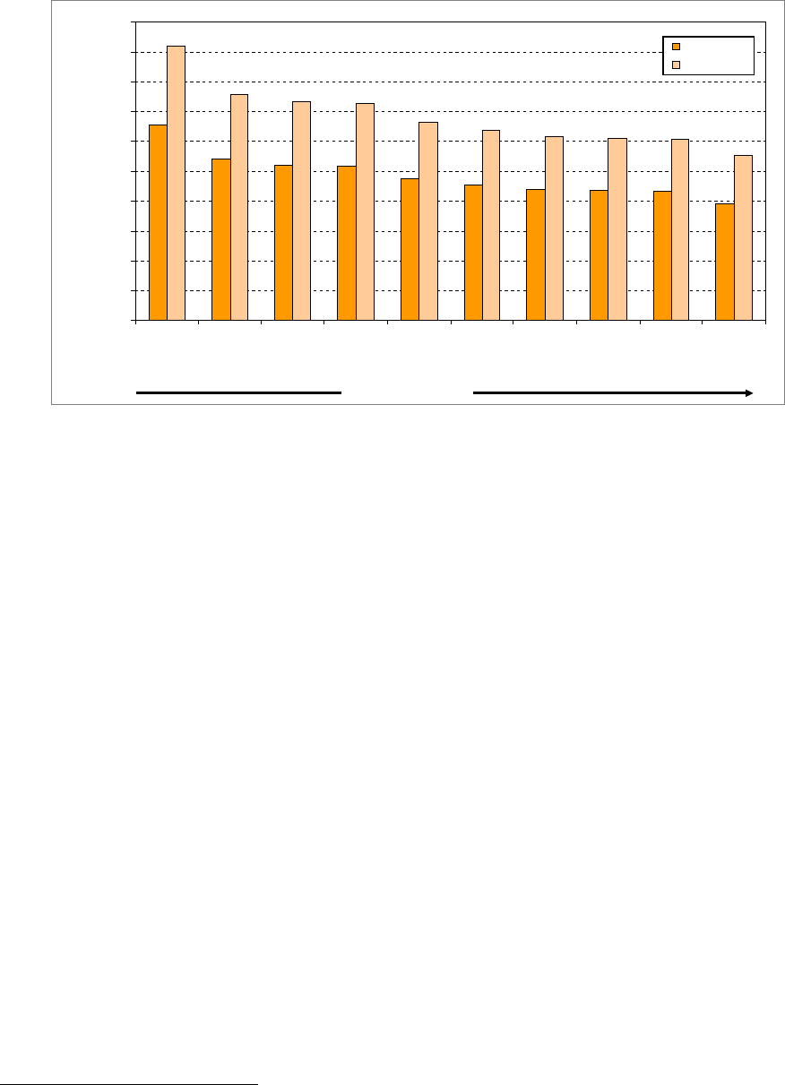
51
Figure 3.1. LCOE for residential PV systems in several U.S. cities in 2008, with and without the
federal investment tax credit (NREL 2009a)
31
The LCOEs of commercial and utility-scale PV systems are generally lower than those of
residential PV systems located in the same region. Installed and O&M costs per watt tend to
decrease as PV system size increases owing to more advantageous economies of scale and other
factors (see Section 3.6 on PV Installation Cost Trends and Section 3.7 on PV Operations and
Maintenance). In addition, larger, optimized, better-maintained PV systems can produce
electricity more efficiently and consistently.
3.2. Solar Resource and Capacity Factor, PV and CSP
Of all the renewable resources, solar is by far the most abundant. With 162,000 terawatts
reaching Earth from the sun, just 1 hour of sunlight could theoretically provide all of society’s
energy needs for 1 year.
3.2.1. Solar Resource for PV
Photovoltaics can take advantage of direct and indirect (diffuse) insolation, whereas CSP is
designed to use only direct insolation. As a result, PV modules need not directly face and track
incident radiation as CSP systems must do. This has enabled PV systems to have broader
geographical application than CSP.
Figure 3.2 illustrates the photovoltaic solar resource in the United States, Germany, and Spain
for a flat-plate PV collector tilted south at latitude. Solar resources across the United States are
mostly good to excellent, with solar insolation levels ranging from about 1,000–2,500
31
Assumptions for Figure 3.1: residential market, 30-year analysis period, 30-year mortgage, 100% financed, 6% interest rate,
6% discount rate, marginal tax rate 35%, installed cost $7.5/W, $300 inverter replacement at year 10, $280 inverter replacement
at year 20, panel degradation 0.5%/year, ITC covers 30% of initial cost, no state or local incentives.
$0.00
$0.05
$0.10
$0.15
$0.20
$0.25
$0.30
$0.35
$0.40
$0.45
$0.50
Seattle,
WA
Chicago, IL NYC, NY Washington
D.C.
Miami, FL Dallas, TX San
Francisco,
CA
Denver, CO Los
Angeles,
CA
Phoenix,
AZ
Levelized Cost of Energy (U.S.$/kWh)
W ith ITC
Without ITC
Increasing insolation
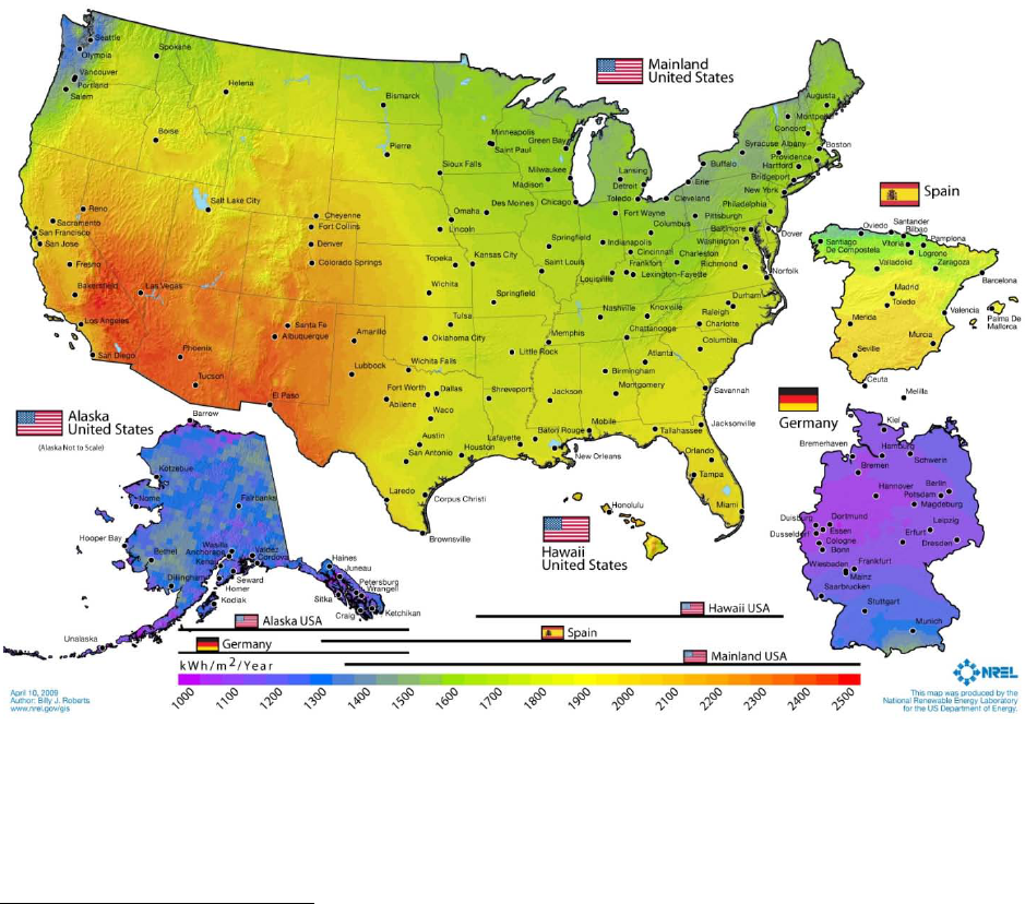
52
kWh/m
2
/year. The southwest U.S. is at the top of this range, while only Alaska and part of
Washington are at the low end. The range for the mainland United States is about 1,350–2,500
kWh/m
2
/year. The U.S. solar insolation level varies by about a factor of 2; this is considered
relatively homogeneous compared to other renewable energy resources.
As is evident from the map, the solar resource in the United States is much higher than in
Germany, and the southwest United States has better resource than southern Spain. Germany’s
solar resource has about the same range as Alaska’s, at about 1,000–1,500 kWh/m
2
/year, but
more of Germany’s resource is at the lower end of that range. Spain’s solar insolation ranges
from about 1,300–2,000 kWh/m
2
/year, which is among the best solar resource in Europe.
Figure 3.2 Photovoltaic solar resource for the United States, Spain, and Germany
32
(NREL 2009d)
Solar PV resource maps are typically provided for horizontal flat-plate PV collectors versus flat-
plate collectors tilted south at latitude. A horizontally oriented module produces less energy per
32
Annual average solar resource data are for a solar collector oriented toward the south at tilt = local latitude. The
data for Hawaii and the 48 contiguous states are derived from a model developed at SUNY/Albany using
geostationary weather satellite data for the period 1998–2005. The data for Alaska were derived by NREL in 2003
from a 40-km satellite and surface cloud cover database for the period 1985–1991. The data for Germany and Spain
were acquired from the Joint Research Centre of the European Commission and capture the yearly sum of global
irradiation on an optimally inclined surface for the period 1981–1990. State and countries are shown to scale, except
for Alaska.

53
unit of module power than the same module tilted south or equipped with a system that tracks the
sun. However, horizontal PV systems can be beneficial when land constraints become a
significant factor, because they have a greater energy density per unit of land area than tilted or
tracking systems. For a fixed land area, more electricity can be generated from a horizontal PV
system than from a tilted or tracking system owing to space needed to avoid self-shading and to
allow for maintenance. On flat commercial roofs, it is cheaper to install flat or nearly flat systems
(Denholm and Margolis 2008b).
The total land area suitable for PV is enormous and will not limit PV deployment. For example,
a current estimate of the total roof area suitable for PV in the United States is approximately
6 billion square meters, even after eliminating 35% to 80% of roof space to account for panel
shading (e.g., by trees) and suboptimal roof orientations. With current PV performance, this area
has the potential for more than 600 GW of capacity, which could generate more than 20% of
U.S. electricity demand. Beyond rooftops, there are many opportunities for installing PV on
underutilized real estate such as parking structures, awnings, airports, freeway margins, and
farmland set-asides. The land area required to supply all end-use electricity in the United States
using PV is about 0.6% of the country's land area (181 m
2
per person) or about 22% of the
“urban area” footprint (Denholm and Margolis 2008c).
3.2.2 Solar Resource for CSP
The geographic area that is most suitable for concentrating solar power is smaller than for PV
because CSP uses only direct insolation. In the United States, the best location for CSP is the
Southwest. Globally, the most suitable sites for CSP plants are arid lands within 35° north and
south of the equator. Figure 3.3 shows the direct-normal solar resource in the southwestern
United States, which includes a detailed characterization of regional climate and local land
features; red indicates the most intense solar resource, and light blue indicates the least intense.
Figure 3.4 shows locations in the southwestern United States with characteristics ideal for CSP
systems, including direct-normal insolation greater than 6.75 kWh/m
2
/day, a land slope of less
than 1°, and at least 10 km
2
of contiguous land that could accommodate large systems (Mehos
and Kearney 2007).
After implementing the appropriate insolation, slope, and contiguous land area filters,
53,900 square miles are available in the seven states considered to be CSP compatible:
California, Arizona, New Mexico, Nevada, Colorado, Utah, and Texas. Table 3.1 summarizes
the land area in these states that is ideally suited to CSP. This relatively small land area amounts
to nearly 6,900 GW of resource potential and more than 16 million GWh of generating capacity,
assuming a capacity factor between 25% and 50% (see Section 3.2.3) (Mehos and Kearney 2007,
Andraka 2008). This is quadruple the annual U.S. electricity generation of about 4 million
GWh.
33
33
EIA Net Generation by Energy Source: Total (All Sectors), rolling 12 months ending in June 2009
www.eia.doe.gov/cneaf/electricity/epm/table1_1.html.
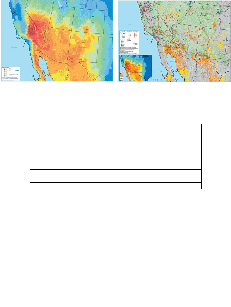
54
Figure 3.3. Direct-normal solar resource in the
U.S. Southwest
(Mehos and Kearney 2007)
Figure 3.4. Direct-normal solar radiation in the
U.S. Southwest, filtered by resource, land use,
and topography
(Mehos and Kearney 2007)
Table 3.1. Ideal CSP Land Area and Resource Potential in Seven Southwestern States
34
State
Available Area (square miles)
Resource Potential (GW)
Arizona
19,300
2,468
California
6,900
877
Colorado
2,100
272
Nevada
5,600
715
New Mexico
15,200
1,940
Texas
1,200
149
Utah
3,600
456
Total
53,900
6,877
Mehos and Kearney 2007
3.2.3 Capacity Factor, PV and CSP
Capacity factor is the ratio of an energy-generation system's actual energy output during a given
period to the energy output that would have been generated if the system ran at full capacity for
the entire period. For example, if a system ran at its full capacity for an entire year, the capacity
factor would be 100% during that year. Because PV and CSP generate electricity only when the
sun is shining, their capacity factors are reduced because of evening, cloudy, and other low-light
periods. This can be mitigated in part by locating PV and CSP systems in areas that receive high
levels of annual sunlight. The capacity factor of PV and CSP systems is also reduced by any
necessary downtime (e.g., for maintenance), which is also the case for other generation
technologies.
For PV, electricity generation is maximized when the modules are normal (i.e., perpendicular) to
the incident sunlight. Variations in the sun's angle that are due to the season and time of day
reduce the capacity factor of fixed-orientation PV systems. This can be mitigated in part by
34
CSP power plants require about 5 acres of land area per MW of installed capacity. Electricity generation for a CSP plant can be
estimated by assuming an average annual solar capacity factor of 25% to 50%, depending on the amount of thermal storage.
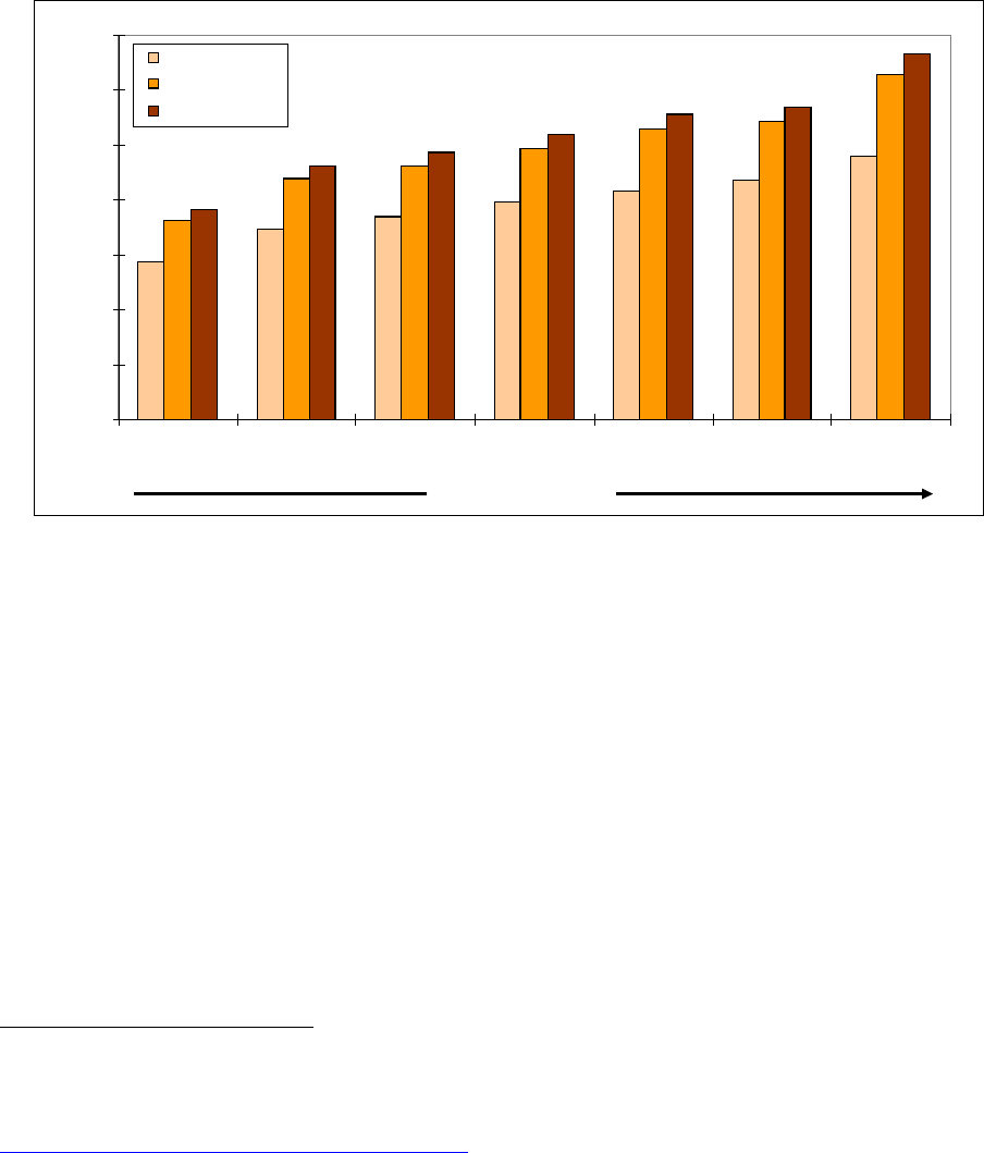
55
tilting stationary PV modules to maximize annual sunlight exposure or by incorporating one- or
two-axis solar tracking systems, which rotate the modules to capture more normal sunlight
exposure than is possible with stationary modules. Figure 3.5 shows the effect of insolation and
use of tracking systems on PV capacity factors. Fixed tilt (at latitude) capacity factors are 14%–
24% for Seattle to Phoenix, whereas 1- and 2-axis tracking systems result in higher ranges.
Analysts sometimes use 18% or 19% for an average U.S. PV capacity factor.
35
Figure 3.5. PV capacity factors varying by insolation and use of tracking systems
(NREL 2009b)
36
The most recently built CSP trough, tower, and dish-engine systems have AC capacity factors in
the mid-20% range. With 6 hours of thermal storage, capacity factors increase to about 40%, and
additional increases in thermal storage will enable capacity factors and dispatchability (the
ability to increase or decrease electricity generation on demand) to increase even more.
3.3 PV Cell, Module, and System Efficiency
In addition to the solar resource and capacity factor discussed above, the amount of electricity
produced by PV systems depends primarily on the following factors:
• Cell type and efficiency
• Module efficiency
• System efficiency
• Module reliability.
35
These are DC capacity factors, i.e., based on the DC rating of a PV system and taking into account inverter and other system
losses. By definition, they are lower than an AC capacity factor, which is how fossil, nuclear, and CSP plants are rated and thus
are not directly comparable to more traditional AC capacity factors.
36
Capacity factors were estimated using data from NREL’s PVWatts, a performance calculator for on-grid PV systems:
http://rredc.nrel.gov/solar/codes_algs/PVWATTS/version1/. The capacity factors shown here reflect an overall derate factor of
0.77, with the inverter and transformer component of this derate being 0.92, the defaults used in PVWatts. The array tilt is at
latitude for the fixed tilt systems, the default in PVWatts.
24%
22%
21%
20%
18%
17%
14%
31%
27%
26%
25%
23%
22%
18%
33%
28%
28%
26%
24%
23%
19%
0%
5%
10%
15%
20%
25%
30%
35%
Seattle, WA Chicago, IL Boston, MA Miami, FL Fort Worth,
TX
Los Angeles,
CA
Phoenix, AZ
Capacity Factor
Fixed Tilt
1-Axis Tracking
2-Axis Tracking
Increasing insolation
56
This section discusses the efficiency of PV cells, modules, and systems. Module reliability is
discussed in the next section.
3.3.1 PV Cell Type and Efficiency
Two categories of PV cells are used in most of today's commercial PV modules: crystalline
silicon and thin film. The crystalline silicon category, called first-generation PV, includes
monocrystalline and multicrystalline PV cells, which are the most efficient of the mainstream PV
technologies and accounted for about 84% of PV produced in 2008 (Bartlett et al. 2009). These
cells produce electricity via crystalline silicon semiconductor material derived from highly
refined polysilicon feedstock. Monocrystalline cells, made of single silicon crystals, are more
efficient than multicrystalline cells but are more expensive to manufacture.
The thin-film category, called second-generation PV, includes PV cells that produce electricity
via extremely thin layers of semiconductor material made of amorphous silicon (a-Si), copper
indium diselenide (CIS), copper indium gallium diselenide (CIGS), or cadmium telluride (CdTe).
Another PV cell technology (also second generation) is the multijunction PV cell. Multijunction
cells use multiple layers of semiconductor material (from the group III and V elements of the
periodic table of chemical elements) to absorb and convert more of the solar spectrum into
electricity than is converted by single-junction cells. Combined with light-concentrating optics
and sophisticated sun-tracking systems, these cells have demonstrated the highest sunlight-to-
electricity conversion efficiencies of any PV technologies, in excess of 40%.
Various emerging technologies, known as third-generation PV, could become viable commercial
options in the future, either by achieving very high efficiency or very low cost. Examples include
dye-sensitized and organic PV cells, which have demonstrated relatively low efficiencies to date
but offer the potential for substantial manufacturing cost reductions.
The efficiencies of all PV cell types have improved over the past several decades, as illustrated
in Figure 3.6, which shows the best research-cell efficiencies from 1975 to 2008. The highest-
efficiency research cell shown is a multijunction concentrator at 41.6% efficiency. Other
research-cell efficiencies illustrated in the figure range from 20% to almost 28% for crystalline
silicon cells, 12% to almost 20% for thin film, and about 5% and to 11% for the emerging PV
technologies organic cells and dye-sensitized cells, respectively.
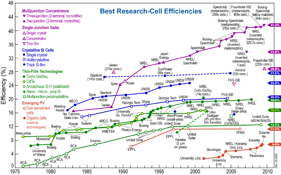
57
Figure 3.6. Best research cell efficiencies 1975–2009
(Kazmerski 2009)
3.3.2 PV Module Efficiency
The cells described in Figure 3.6 were manufactured in small quantities under ideal laboratory
conditions and refined to attain the highest possible efficiencies. The efficiencies of mass-
produced cells are always lower than the efficiency of the best research cell. Further, the
efficiency of PV modules is lower than the efficiency of the cells from which they are made.
In 2008, the typical efficiency of crystalline silicon-based PV modules ranged from 13.5% for
multicrystalline modules to 17.5% for high-efficiency monocrystalline modules (Mehta and
Bradford 2009). For thin-film modules, typical efficiencies ranged from 6.5% for a-Si modules
to about 10% for CIGS and CdTe modules (Mehta and Bradford 2009).
Figure 3.7 shows best-in-class module efficiencies from 1999 to 2008, with the best crystalline
silicon efficiencies at 17%–19% and the best thin-film efficiencies at 7%–11% in 2008.
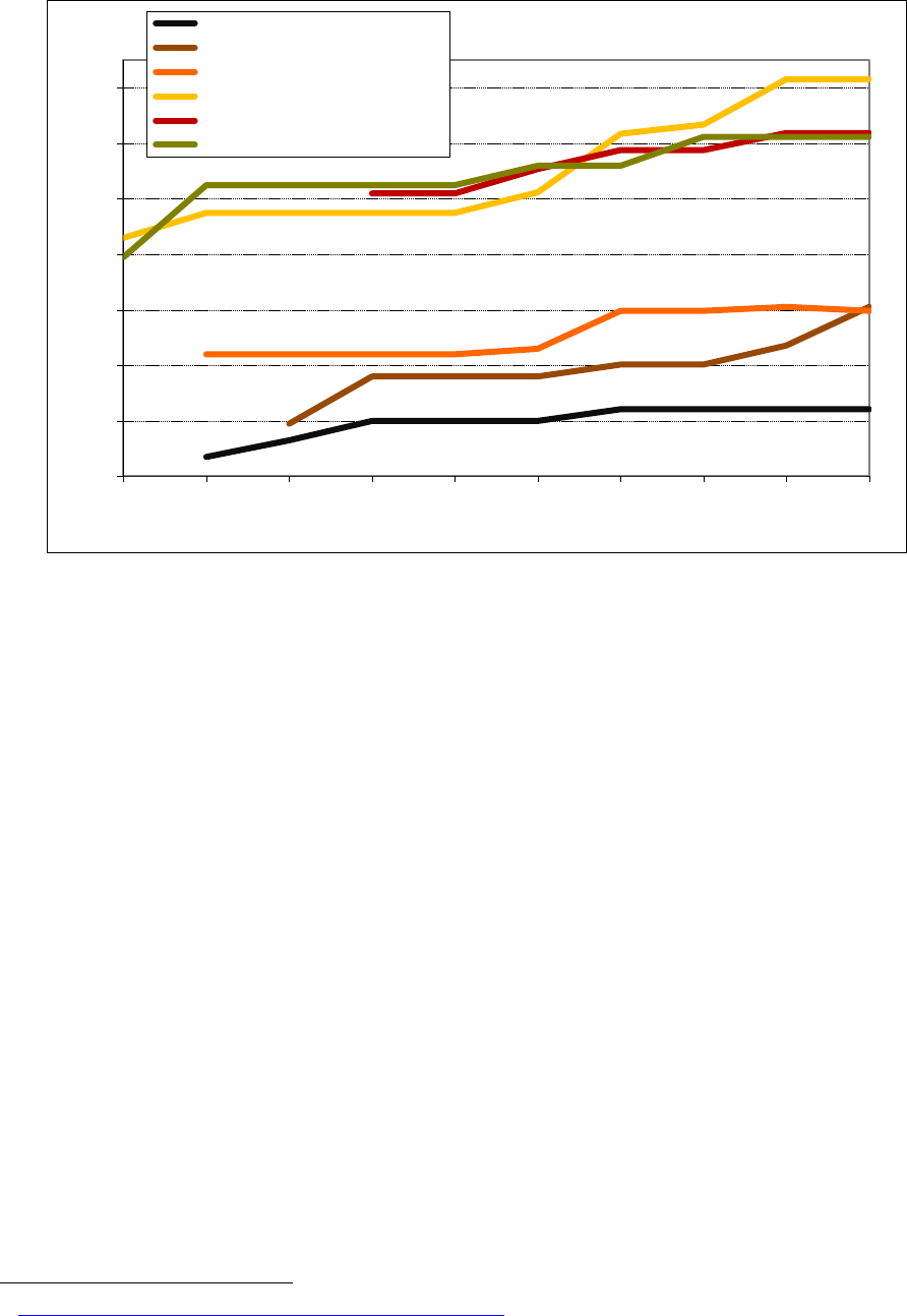
58
Figure 3.7. Best-in-class commercial module efficiencies, 1999–2008, compiled from module
survey data (Kreutzmann 2008, Photon International 1999–2008)
3.3.3 PV System Efficiency and Derate Factor
A PV system consists of multiple PV modules wired together and installed on a building or other
location. The AC output of a PV system is always less than the DC rating, which is due to
system losses.
For grid-connected applications, a PV system includes an inverter that transforms the DC
electricity produced by the PV modules into AC electricity. The average maximum efficiency of
inverters was 95.5% in 2008, up from 94.7% in 2005 (Knoll and Kreutzmann 2008). Other
factors that reduce a PV system's efficiency include dirt and other materials obscuring sun-
collecting surfaces, electrically mismatched modules in an array, wiring losses, and high cell
temperatures. For example, NREL’s PVWatts,
37
3.4 PV Module Reliability
a performance calculator for on-grid PV
systems, uses an overall derate factor of 0.77 as a default, with the inverter component of this
derate being 0.92.
Historic data suggest that reliability is a very important factor when considering the market
adoption of a new technology, especially during the early growth stages of an industry. PV is
currently experiencing unprecedented growth rates. To sustain these growth rates, it is imperative
that manufacturers consider the implications of product reliability.
37
http://rredc.nrel.gov/solar/codes_algs/PVWATTS/version1/
5
7
9
11
13
15
17
19
1999
2000
2001
2002
2003
2004
2005
2006
2007
2008
Efficiency (%)
a-Si
CdTe
CIS
Monocrystalline
HIT (monocrystalline & a-Si)
Multicrystalline
59
Today’s PV modules usually include a 25-year warranty. Standard warranties guarantee that
output after 25 years will be at least 80% of rated output. This is in line with real world
experience and predicted performance from damp-heat testing of modules (Wohlgemuth et al.
2006).
Manufacturers in the United States, Japan, and the European Union currently implement
qualification standards and certifications that help to ensure that PV systems meet reliability
specifications. There have been efforts to bring reliability standards to Chinese manufacturers as
well, considering their rapid growth in the PV market. DOE has been a leader in engaging
Chinese manufacturers in discussions on reliability standards and codes by organizing a series of
reliability workshops and conferences in China. The global PV community realizes that if
reliability standards are not quickly implemented among the fastest-growing producers,
consumers left with high-maintenance installations could negatively impact market adoption of
PV modules both now and in the future.
3.5 PV Module Price Trends
Photovoltaic modules have experienced significant improvements and cost reductions over the
last few decades, and the market for PV modules has undergone unprecedented growth in recent
years owing to government policy support and other financial incentives encouraging the
installation of (primarily grid-connected) PV systems. Although PV module prices increased in
the past several years, prices have been falling steadily over the past few decades and began
falling again in 2008. This is illustrated in Figure 3.8, which presents average global PV module
selling prices for all PV technologies.
Although global average prices provide an index for the PV industry overall, a few caveats are in
order. First, the PV industry is dynamic and rapidly changing, with advances in cost reductions
for segments of the industry masked by looking at average prices. For example, thin-film PV
technologies are achieving manufacturing costs and selling prices significantly lower than for
crystalline silicon modules. See Table 3.2 (at the end of Section 3.5) for comparison of module
costs and prices for various PV technologies. Applications such as large ground-mounted PV
systems, for which deployment is increasing, and applications in certain countries and locations,
accrue cost advantages based on factors such as economies of scale and the benefits of a more
mature market (some of this is captured in Section 3.6 on PV installation cost trends). Finally,
historical trends may not provide an accurate picture going forward, as new developments
continue to change the PV industry landscape.
Figure 3.8 shows average global PV module selling prices at the factory gate (i.e., prices do not
include charges such as delivery and subsequent taxes), as obtained from sample market
transactions. As stated earlier, these prices are averages over all PV module technologies
including thin film, for PV power modules greater than 75 W in size and purchased in relatively
small quantities. Excluded from this category are smaller PV modules, consumer indoor PV
(e.g., for calculators and watches), and large (e.g., greater than 150 W) standard modules sold in
large quantities (e.g., 500–1,000-unit minimums) in the unrestricted international commodity
market. The large-module/large-quantity category has been increasing in market share in recent
years and constituted more than half of module sales in 2008. In 2008, the average price per watt
for the large-module/large-quantity category was 11% lower than for the power module category
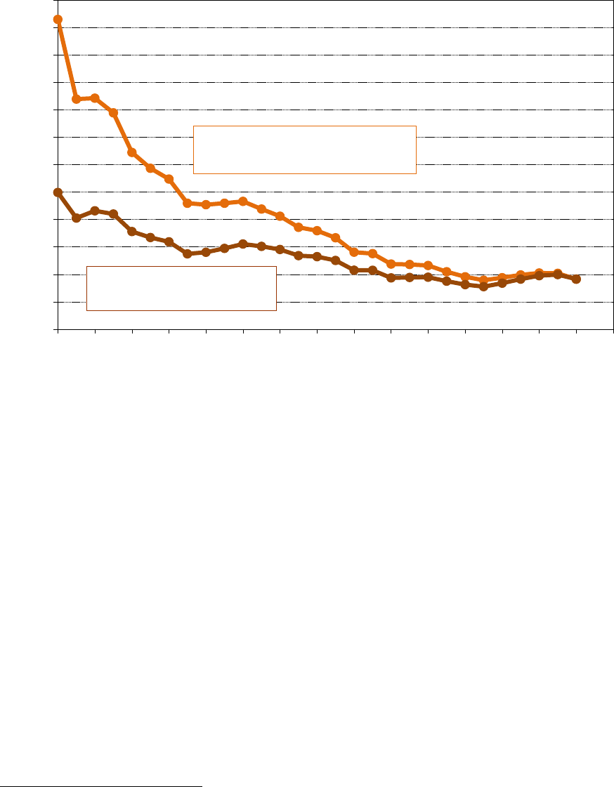
60
shown in Figure 3.8. The current/nominal prices shown in the figure are actual prices paid in the
year stated. The 2008/real prices are adjusted for inflation (indexed to 2008 U.S. dollars).
Figure 3.8. Global, average PV module prices, all PV technologies, 1980–2008
(Mints 2006, Mints 2009, U.S. Bureau of Economic Analysis 2009)
38
39
PV module prices experienced significant drops in the mid-1980s resulting from increases in
module production and pushes for market penetration during a time of low interest in renewable
energy. Prices dropped by more than $10/W (in real 2008$) between the early- to mid-1980s.
The price of PV by 1987 was approximately $9/W. PV prices then experienced an increase from
1988 through 1990 as the supply of PV modules diminished because of a limitation in the
availability of silicon wafers. For the first time in a decade, the market was limited by supply
rather than demand. Prices then dropped significantly from 1991 to 1995 because of increases in
manufacturing capacity and a worldwide recession that slowed PV demand. Module prices
continued to fall, although at a slower rate from 1995 to 2003, which was due to global increases
in module capacities and a growing market. By 2000, module prices were below $5/W, reaching
a low of $3/W in 2003 (Mints 2009).
Prices began to increase from 2003 to 2006 as European demand, primarily from Germany and
Spain, experienced high growth rates after feed-in tariffs and other government incentives were
adopted. Also contributing to the price increases was an imbalance between polysilicon supply
and demand from around 2004 to mid-2008. Higher prices were sustained until the third quarter
of 2008 when the global recession reduced demand, polysilicon supply constraints eased, and
38
Current/nominal data provided by Mints, then adjusted for inflation using GDP deflator from the U.S. Bureau of
Economic Analysis.
39
See Table 3.2 later in this section for comparison of module costs and prices for various PV technologies.
0
2
4
6
8
10
12
14
16
18
20
22
24
1980 1982 1984 1986 1988 1990 1992 1994 1996 1998 2000 2002 2004 2006 2008 2010
Average Module Price (Current and 2008$/W)
2008/Real U.S.$/W
(Mints 2009, U.S. BEA 2009)
Current/Nominal U.S.$/W
(Mints 2009)

61
module supply increased. For the first time since 2003, average module prices declined to
$3.65/W, down from approximately $4/W in 2007 (in real 2008$).
Module prices vary considerably by technology (Table 3.2), influenced by variations in
manufacturing cost and sunlight-to-electricity conversion efficiency, among other factors.
Manufacturing cost is the reference point against which a manufacturer sets its profit margin; the
closer the selling price is to the manufacturing cost, the lower the profit margin and vice versa.
Higher conversion efficiency generally commands a price premium. This is because higher-
efficiency modules require less installation area per watt of electricity production and incur
lower balance-of-systems costs (i.e., wiring, racking, and other system installation costs) per watt
than lower-efficiency modules. The current estimated effect is a $0.10 increase in price per 1%
increase in efficiency; for example, all else being equal, a 20%-efficient module would cost
about $1 more per watt than a 10%-efficient module (Mehta and Bradford 2009).
Table 3.2. Module Price, Manufacturing Cost, and Efficiency Estimates by Technology, 2008
Technology
Price
(2008 $/Wp)
Manufacturing Cost
(2008 $/Wp)
Conversion
Efficiency
High-efficiency monocrystalline silicon
$3.83
$2.24
17.5%
Multicrystalline silicon
$3.43
$2.12–$3.11
40
13.5%
Amorphous silicon (a-Si) thin film
$3.00
$1.80
6.5%
Copper indium diselenide/copper indium
gallium diselenide (CIS/CIGS) thin film
$2.81 $1.26 10.2%
Cadmium telluride (CdTe) thin film
$2.51
$1.25
10.0%
Mehta and Bradford 2009
3.6 PV Installation Cost Trends
41
Lawrence Berkeley National Laboratory (LBNL) has collected project-level installed system cost
data for grid-connected, customer-sited PV installations in the Unites States from a number of
solar incentive program administrators (Wiser et al. 2009). The dataset currently includes
approximately 52,000 PV systems installed in 16 states between 1998 and 2008 and totals
565 MW, or 71% of all grid-connected PV capacity installed in the United States through 2008.
Below are trends related to the installed system cost of the PV projects in the LBNL database. In
all instances, installed costs are expressed in terms of real 2008 dollars and represent the cost to
the consumer before receipt of any grant or rebate. PV capacity is expressed in terms of the rated
module direct-current (DC) power output under Standard Test Conditions. Note that the
terminology “installed cost” in this report represents the price paid by the end-user/customer.
This should not be confused with the term “cost” as used in other contexts to refer to the cost to a
company before a product is priced for a market or end user.
40
The range in manufacturing cost for multicrystalline silicon includes $2.12 for global, vertically integrated PV module
manufacturers, $2.74 for European manufacturers, and $3.11 for Asian manufacturers, with much of the difference being due to
the price of polysilicon feedstock paid in 2008 by each type of producer.
41
This section on PV installation cost trends was provided by Wiser et al. 2009, of LBNL, before the publication of their full
report, “Tracking the Sun II. The Installed Cost of Photovoltaics in the U.S. from 1998-2008,”
http://eetd.lbl.gov/ea/EMS/re-
pubs.html, with the full reference provided in the Chapter 3 references. Note that some of the numbers presented in this section
may be slightly different from numbers in the published LBNL report, though the numbers stated in the text corresponding to the
first figure of this section, Figure 3.9, are the same.

62
Figure 3.9 presents the average installed cost from 1998 to 2008 for the entire sample of projects.
Capacity-weighted average costs declined from $10.8/W in 1998 to $7.5/W in 2008. This
represents an average annual reduction of $0.3/W (i.e., a drop of 3.6% per year in real
dollars). Figure 3.9 also shows that the distribution in installed costs, indicated by the standard
deviation bars, has narrowed over time, suggesting a maturing market with converging costs.
Both average installed costs and the distribution in installed costs, however, remained relatively
stable from 2005 to 2007. Costs declined from 2007 to 2008 at the historical average pace of
$0.3/W.
Figure 3.9. Installed cost trends over time
(Wiser et al. 2009)
The long-term decline in installed costs from 1998 to 2008 is attributable primarily to a drop in
non-module costs. Non-module costs can include inverters, other hardware, labor, permitting and
fees, shipping, overhead, and profit. As shown in Figure 3.10, the average non-module costs
(calculated as the difference between average total installed cost and a module price index
42
)
declined from approximately $5.9/W in 1998 to $3.8/W in 2008, a drop of $2.1/W. By
comparison, module prices dropped by only $1.3/W over this 11-year period. From 2005 through
2008, however, non-module costs remained relatively stable; in fact, from 2007 to 2008, non-
module costs increased slightly while module costs declined by $0.5/W.
42
The global, average annual price of power modules published by Navigant Consulting is used (see the previous section,
Section 3.5 on PV Module Price Trends).
$0
$2
$4
$6
$8
$10
$12
$14
$16
1998
n=39
0.2 MW
1999
n=178
0.7 MW
2000
n=213
0.9 MW
2001
n=1239
4.8 MW
2002
n=2290
12 MW
2003
n=3334
31 MW
2004
n=5498
46 MW
2005
n=5193
60 MW
2006
n=8681
90 MW
2007
n=12107
123 MW
2008
n=13013
195 MW
Installation Year
Installed Cost (2008$/W)
Capacity-Weighted Average
Simple Average +/- Std. Dev.
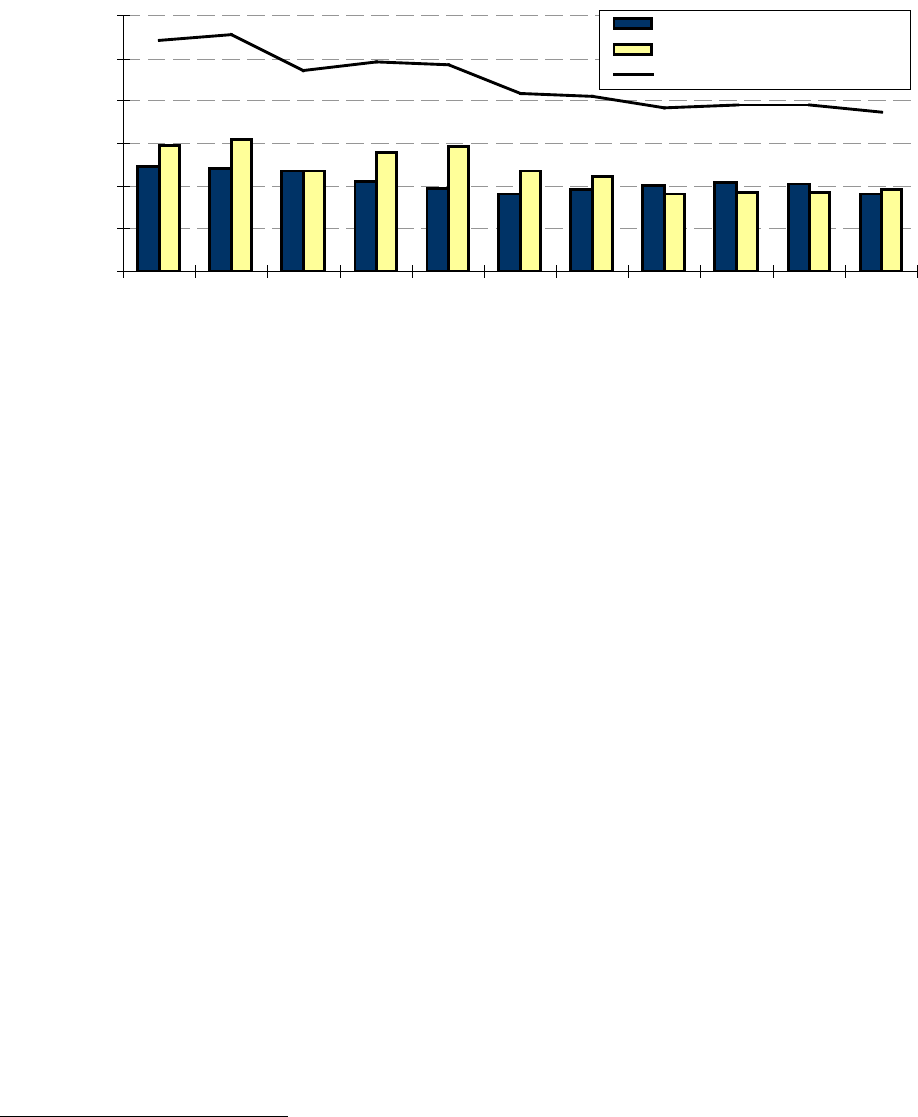
63
Figure 3.10. Module and non-module cost trends over time
(Wiser et al. 2009)
Although experience to date confirms that significant cost reductions occurred in the United
States from 1998 through 2008, international experiences suggest that further cost reductions are
possible and may accompany increased market size. Figure 3.11 compares installed costs in
Japan, Germany, and the United States, focusing specifically on 2–5-kW residential systems
installed in 2007 (and excluding sales tax).
43
Among these systems, average installed costs were
substantially lower in Japan and Germany ($6.1/W and $6.8/W, respectively) than in the United
States ($8.1/W). These differences may partly reflect the much greater cumulative grid-
connected PV capacity in Japan and Germany (about 1.8 GW and 3.8 GW, respectively) at the
end of 2007 compared to just 0.5 GW in the United States. However, it is also evident that larger
market size alone does not account for all of the variation; installed costs are higher in Germany
than in Japan, despite Germany’s grid-connected PV capacity being substantially greater.
44
43
Year 2008 data are not yet available for Germany and Japan.
44
One potential explanation for the relatively low residential PV costs in Japan is that a large portion of the
residential PV market consists of pre-fabricated homes that include PV as a standard feature. More generally,
installed costs may differ among countries as a result of a wide variety of factors, including differences in module
prices, technical standards for grid-connected PV systems, installation labor costs, procedures for receiving
incentives and interconnection approvals, and the degree to which components are manufactured locally (thereby
reducing transportation costs).
$0
$2
$4
$6
$8
$10
$12
1998
n=39
0.2 MW
1999
n=178
0.7 MW
2000
n=213
0.9 MW
2001
n=1239
4.8 MW
2002
n=2290
12 MW
2003
n=3334
31 MW
2004
n=5498
46 MW
2005
n=5193
60 MW
2006
n=8681
90 MW
2007
n=12107
123 MW
2008
n=13013
195 MW
Installation Year
Capacity-Weighted Average
Installed Cost (2008$/W)
Global Module Price Index
Non-Module Cost (calculated)
Total Installed Cost
Note: Non-module costs are calculated as the reported total installed costs minus the global module price index.
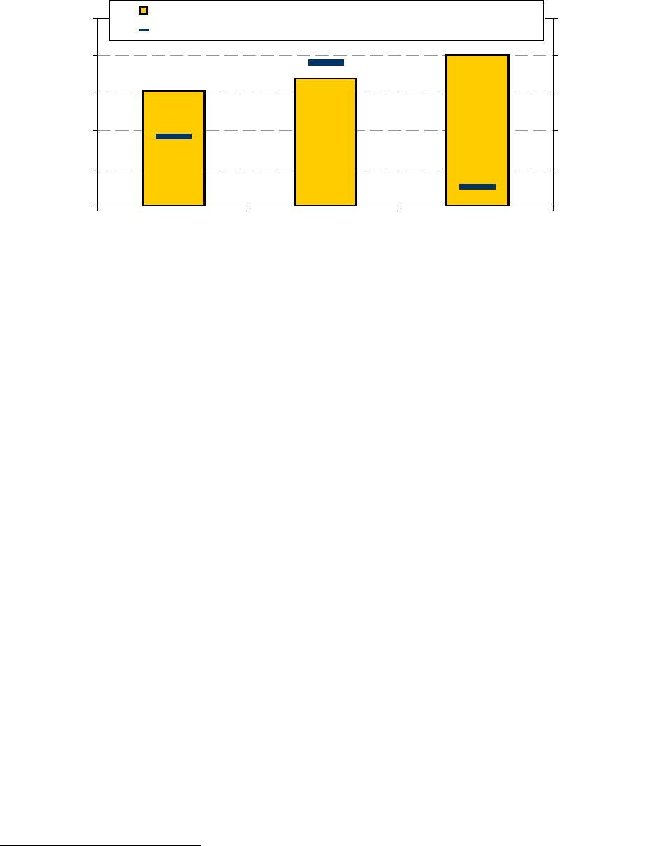
64
Figure 3.11. Average installed cost of residential systems completed in 2007
in Japan, Germany, and the United States
(Wiser et al. 2009)
The United States is not a homogenous PV market, as evidenced by Figure 3.12, which compares
the average installed cost of PV systems <10 kW completed in 2008 across 16 states. Average
costs range from a low of $7.3/W in Arizona to a high of $10.5/W in Maryland. Differences in
the average installed cost across these states may, in part, reflect the differing size and maturity
of their PV markets. Specifically, the largest PV markets in the United States (California, New
Jersey, and Colorado
45
) have among the lowest average costs, and a number of smaller but
relatively mature markets (Arizona, Connecticut, and Massachusetts) also have low costs. In
addition, 8 of the 16 states shown in the Figure 3.12 (Arizona, Connecticut, Massachusetts,
Minnesota, New Jersey, New York, Washington, and Vermont) exempted residential PV systems
from state sales tax in 2008, and Oregon has no state sales tax. Sales tax exemptions effectively
reduce post-sales tax installed costs by $0.2–0.4/W, depending on the otherwise applicable sales
tax rate and assuming that PV hardware costs represent approximately 65% of the total installed
cost of residential PV systems (an assumption supported by data presented later in this section).
45
The LBNL dataset does not include data from Colorado’s largest PV incentive program (Xcel Energy’s Solar
Reward’s Program). Thus, the sample of Colorado projects is small, even though the total number of projects
installed in the state in 2008 is relatively large.
$0
$2
$4
$6
$8
$10
Japan Germany United States
Average Residential PV
Installed Cost without Sales
Tax (2008$/W)
0
1,000
2,000
3,000
4,000
5,000
Cumulative Grid-Connected
Capacity through 2007 (MW)
Avg. Installed Cost of Residential Systems in 2007 (left axis)
Cumulative Grid-Connected Capacity through 2007 (right axis)
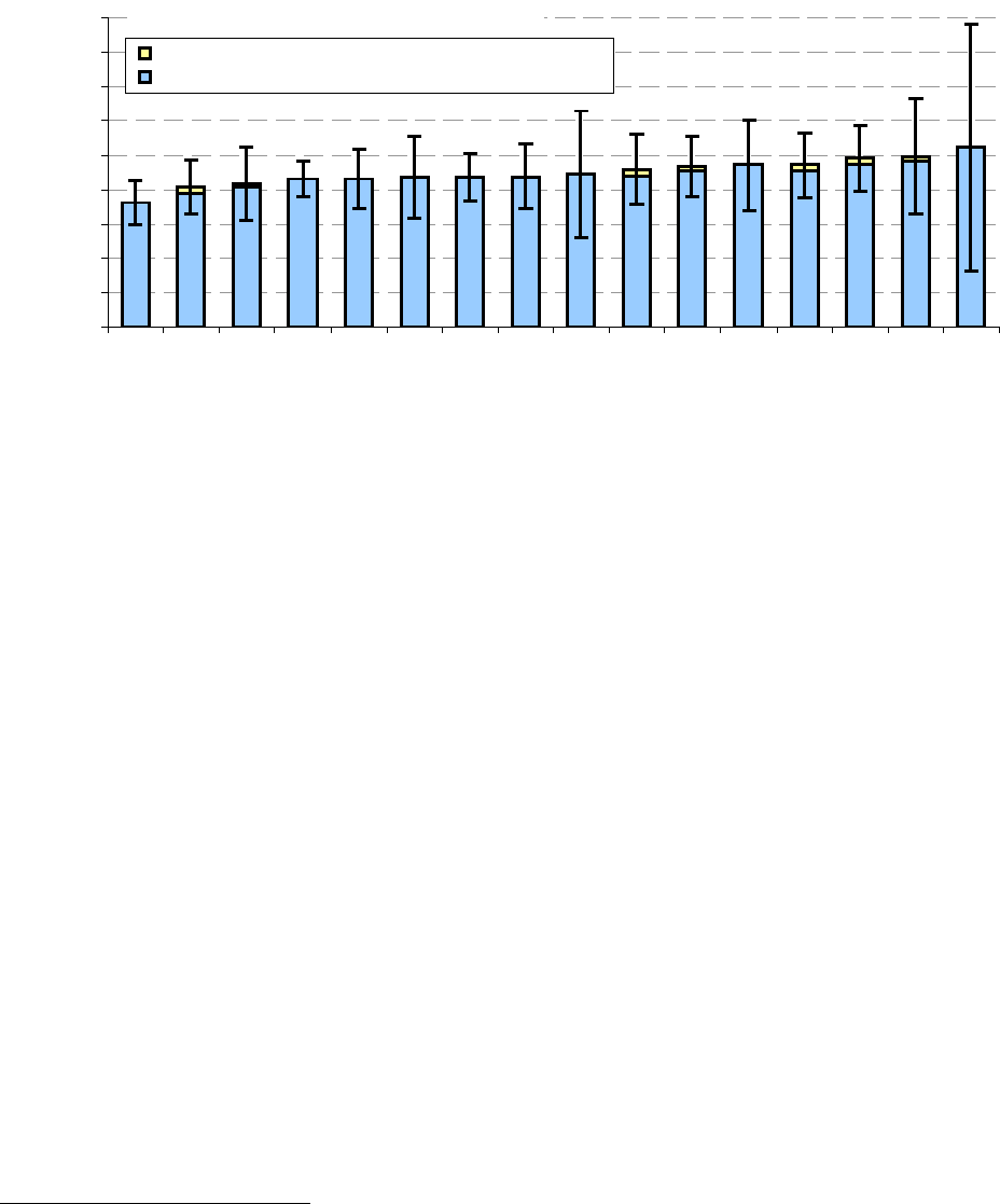
65
Figure 3.12. Variation in installed costs among U.S. states
(Wiser et al. 2009)
The decline in U.S. PV installed costs over time is partly attributable to the fact that PV systems
have gotten larger, on average, and exhibit some economies of scale. As shown in Figure 3.13,
the average size of systems ≤10 kW (a proxy for residential systems) grew from 2.7 kW in 1998
to 4.6 kW in 2008.
46
Similarly, the average size of systems >10 kW (a proxy for non-residential
systems) rose from 25 to 88 kW over the same period, although the trend is notably more uneven
than for the smaller systems. As confirmed by Figure 3.14, installed costs generally decline as
system size increases. In particular, the average installed cost of systems installed in 2008 was
greatest for systems <2 kW, at $9.2/W, dropping to $6.2/W for systems in the 500–750-kW size
range, a decline of approximately $2.6/W, or about 28%.
47
Of interest, however, is that the
economies of scale are not continuous but, rather, are most apparent for systems at the lower and
upper ends of the size spectrum (i.e., for systems in the <5 kW range and the >250 kW range). In
addition, the average cost of systems >750 kW in 2008 was slightly higher than the average cost
of 500–750 kW systems ($7.1/W vs. $6.6/W, respectively), perhaps indicative of a greater
proportion of tracking systems within the larger size range.
46
The data provided by many PV incentive programs did not identify customer type (i.e., residential vs. non-
residential); thus ≤10 kW is used as a proxy for residential systems, recognizing that a non-trivial portion of systems
≤10 kW are, in fact, non-residential.
47
Note that the LBNL data do not include several larger PV systems installed in 2008 including a 2.4-MW plant in
Fontana, CA; a 3.0-MW plant in Fairless Hills, PA; and a 12.6-MW plant in Boulder City, NV. Installed costs for
the CA and NV projects ($4.3/W and $3.2/W, respectively), as reported in press releases, are considerably less than
the average installed costs shown in Figure 8 for customer-sited projects >750 kW.
$0
$2
$4
$6
$8
$10
$12
$14
$16
$18
AZ
n=431
CA
n=8594
CO
n=16
CT
n=249
MA
n=296
NJ
n=690
NY
n=356
OR
n=201
WA
n=6
NV
n=141
MD
n=131
VT
n=89
WI
n=125
PA
n=16
OH
n=18
MN
n=28
Average Installed Cost (2008$/W)
State Sales Tax (if assessed)
Pre-Sales Tax Installed Cost (Avg. +/- Std. Dev.)
Systems <10 kW, Installed in 2008
Note: State Sales Tax and Pre-Sales Tax Installed Costs were calculated from 2008 sales tax rates in each state, accounting
for sales tax exemptions for PV systems. Sales tax was assumed to have been assessed only on hardware costs, which in
turn were assumed to constitute 65% of the total pre-sales-tax installed cost.
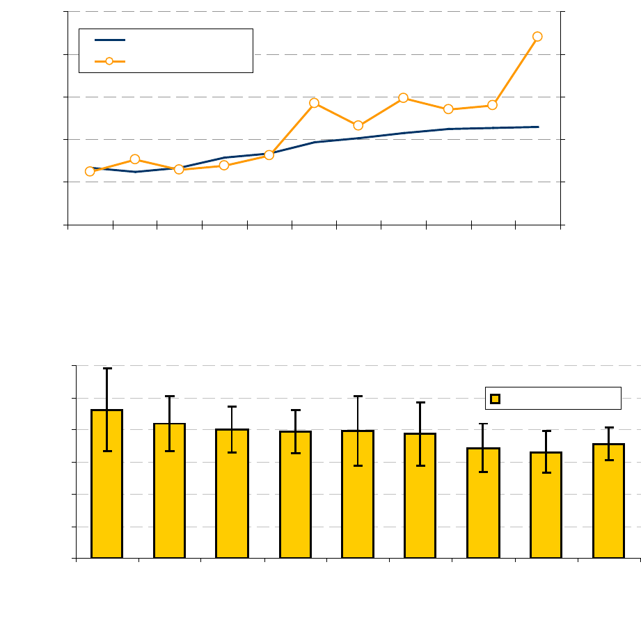
66
Figure 3.13. PV system size trends over time
(Wiser et al. 2009)
Figure 3.14. Variation in installed cost according to PV system size
(Wiser et al. 2009)
In addition to variation across states and system size, installed costs also vary across key market
segments and technology types. Figure 3.15 compares the average installed cost of residential
retrofit and new construction systems completed in 2008, showing separate comparisons for both
rack-mounted and building-integrated photovoltaic (BIPV), and focusing on systems of 1–3 kW,
because that is the size range typical of new construction systems. Rack-mounted systems
installed in residential new construction average $1.2/W less than comparably sized residential
retrofits. For BIPV systems, residential new construction systems average $1.5/W less than
residential retrofits. Figure 3.16 compares installed costs of systems using crystalline silicon
versus thin-film modules, among rack-mounted systems installed in 2008. The data indicate that,
in both the <10-kW and 10–100-kW size ranges, PV systems using thin-film modules were more
0
2
4
6
8
10
1998 1999 2000 2001 2002 2003 2004 2005 2006 2007 2008
Installation Year
Average Size of
Systems (kW)
0
20
40
60
80
100
Average Size of >10 kW
Systems (kW)
≤10 kW (left axis)
>10 kW (right axis)
$0
$2
$4
$6
$8
$10
$12
<2 kW
n=791
1 MW
2-5 kW
n=6349
22 MW
5-10 kW
n=4247
29 MW
10-30 kW
n=1010
14 MW
30-100 kW
n=297
15 MW
100-250 kW
n=147
24 MW
250-500 kW
n=109
37 MW
500-750 kW
n=31
18 MW
>750 kW
n=32
34 MW
System Size Range (kW)
Average Installed Cost (2008$/W)
Avg. +/- Std. Dev.
Systems Installed in 2008
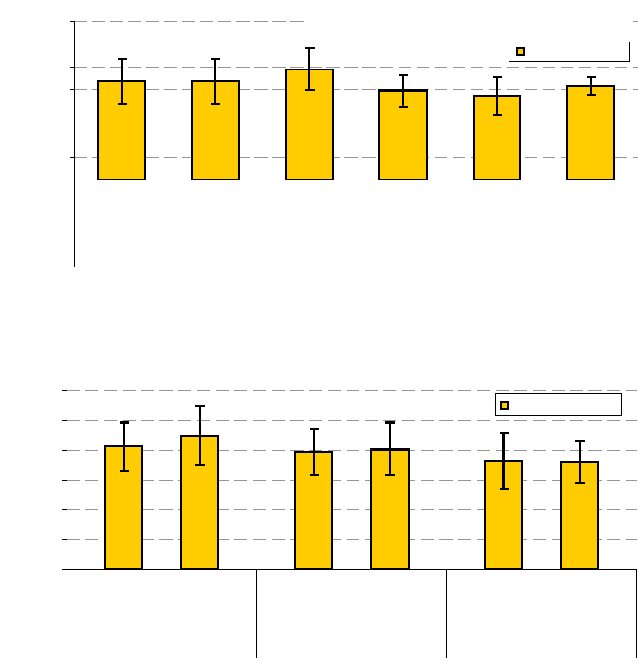
67
costly, on average, than those with crystalline technology, with a difference of $0.8/W in the
<10-kW size range and a somewhat smaller cost differential ($0.3/W) in the 10–100-kW range.
In the >100-kW size range, average installed costs for the two types of systems differed by less
than $0.1/W.
Figure 3.15. Comparison of installed cost for residential retrofit vs. new construction
(Wiser et al. 2009)
Figure 3.16. Comparison of installed cost for crystalline vs. thin-film systems
(Wiser et al. 2009)
Figure 3.10 presents implied module and non-module costs, imputed from data on total installed
cost and a module price index. Figure 3.17, in contrast, presents actual data on module, inverter,
and “other” (e.g., mounting hardware and labor) costs reported to incentive program
$8.7
$8.7
$9.8
$7.9
$7.4
$8.3
$0
$2
$4
$6
$8
$10
$12
$14
All Systems
n=1506
3.6 MW
Rack-Mounted
n=1460
3.5 MW
BIPV
n=41
0.1 MW
All Systems
n=696
1.5 MW
Rack-Mounted
n=336
0.7 MW
BIPV
n=359
0.8 MW
Retrofit New Construction
Average Installed Cost
(2008$/W)
Avg. +/- Std. Dev
Note : The number of rack-mounted systems plus BIPV systems may not sum to the total number of systems, as some
systems could not be identified as either rack-mounted or BIPV.
California CSI, NSHP, and ERP Programs:
1-3 kW Systems Installed in 2008
$7.2
$7.3
$8.1
$7.8
$9.0
$8.2
$0
$2
$4
$6
$8
$10
$12
Crystalline
n=9102
43 MW
Thin-Film
n=678
3.2 MW
Crystalline
n=1091
24 MW
Thin-Film
n=85
2.2 MW
Crystalline
n=242
86 MW
Thin-Film
n=23
7 MW
< 10 kW 10 - 100 kW > 100 kW
Average Installed Cost (2008$/W)
Avg. +/- Std. Dev.
Rack-Mounted Systems Installed in 2008
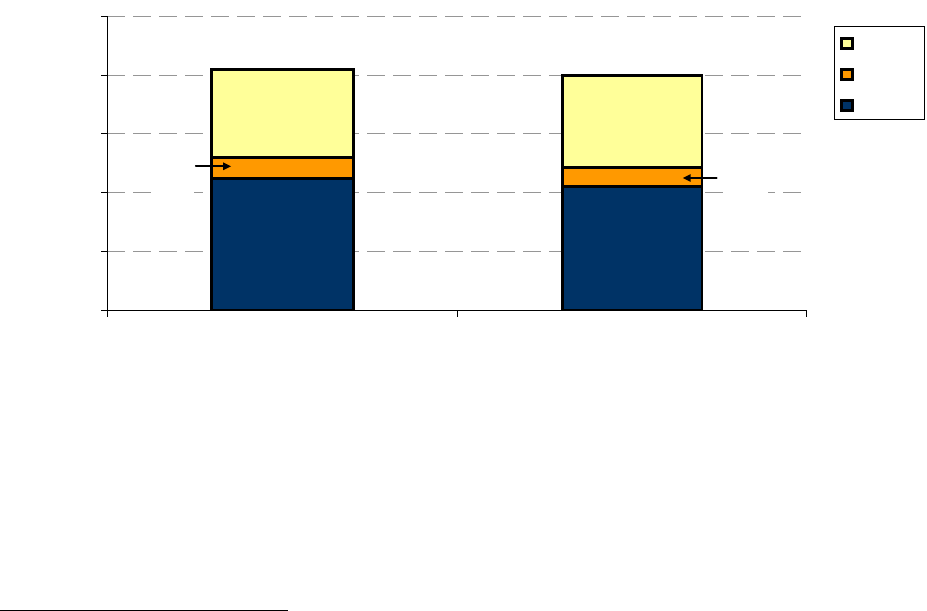
68
administrators, for a limited number of projects installed in 2008.
48
The magnitude of each
component and its relative contribution to total costs are similar for the two system size ranges
shown (<10 kW and 10–100 kW).
49
Modules, on average, represent slightly more than 50% of
total costs, inverters average just under 10% of total costs, and “other” costs make up the
remaining portion.
The component cost breakdown in Figure 3.17 conforms reasonably well to PV installer data
obtained by LBNL in 2008, in which installers shared data on the typical contributions of a
variety of specific cost components, as a percentage of total installed cost (Figure 3.18).
Figure 3.18 also presents the average percentage contribution for each cost component for three
separate PV markets (residential, small commercial, and large commercial).
50
Installers reported
that module costs typically represent approximately 50% of total installed cost, and inverters
represent 6%–7% of total costs, which is generally consistent with the results presented
previously. The results, however, provide a greater level of granularity in understanding the
composition of the remaining costs. In particular, the data indicate that labor and other materials
contribute roughly 10% each. The remaining cost components include overhead, profit, and
regulatory compliance (e.g., permitting, interconnection, rebate application), which represent a
notably greater percentage of total installed costs for residential systems compared with non-
residential systems.
Figure 3.17. Module, inverter, and other costs
(Wiser et al. 2009)
48
Of the 195 MW of 2008 PV installations in the LBNL dataset, incentive program administrators provided module
and inverter cost data for only 2.6 MW (1.3%), which form the underlying data for this figure.
49
Insufficient data were available for systems >100 kW to warrant inclusion in this figure.
50
In total, six installers provided data for residential and large commercial systems, and five installers provided data
for small commercial systems.
$4.5
$4.2
$0.6
$0.7
$3.2
$3.0
(52%)
(55%)
(8%)
(9%)
(40%)
(36%)
$0
$2
$4
$6
$8
$10
< 10 kW
(n=2170)
10 - 100 kW
(n=145)
System Size Range
Average Cost (2008$/W)
Other
Inverter
Module
Systems Installed in 2008
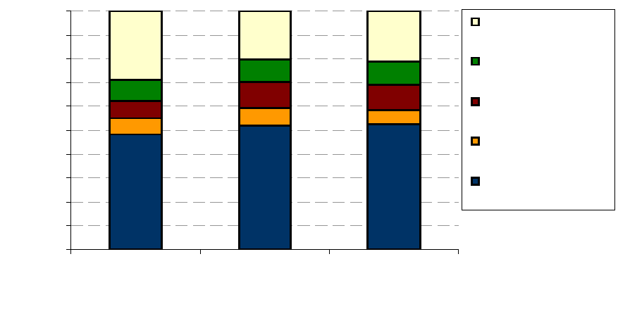
69
Figure 3.18. PV installer data on component costs
(Wiser et al. 2009)
3.7 PV Operations and Maintenance
Operations and maintenance (O&M) is a significant contributor to the lifetime cost of PV
systems, and reducing the O&M costs of system components is an important avenue to reducing
lifetime PV cost. The data, however, are difficult to track, because O&M costs are not as well
documented as other PV system cost elements (which is due in part to the long-term and periodic
nature of O&M).
3.7.1 PV Operations and Maintenance Not Including Inverter Replacement
During the past decade, Sandia National Laboratories has collected O&M data for several types
of PV systems in conjunction with Arizona Public Service (APS) and Tucson Electric Power
(TEP) (Table 3.3). Because O&M data were collected for only 5–6 years in each study, data on
scheduled inverter replacement/rebuilding were not collected; inverters are typically replaced
every 7–10 years. Therefore, the information in Table 3.3 does not include O&M costs
associated with scheduled inverter replacement/rebuilding. This issue is discussed in the next
section of this report.
As shown in Table 3.3, annual O&M costs as a percentage of installed system cost ranged from
0.12% for utility-scale generation to 5%–6% for off-grid residential hybrid systems. The O&M
energy cost was calculated to be $0.004/kWh(ac) for utility-scale generation and $0.07/kWh(ac)
for grid-connected residential systems; note that this is simply annual O&M cost divided by
annual energy output, not LCOE. For all the grid-connected systems, inverters were the major
O&M issue. Following are brief summaries of four recent studies on O&M that provide
additional context.
48%
52%
52%
7%
7%
6%
7%
11%
11%
9%
9%
10%
29%
20%
21%
0%
10%
20%
30%
40%
50%
60%
70%
80%
90%
100%
Residential
(3-5 kW)
Small Commercial
(10-50 kW)
Large Commercial
(>100 kW , roof-
mounted fixed-axis)
Percent of Total Installed Cost
Overhead, Regulatory
Compliance, Other
Installation Labor
Other Materials
Inverter
Module
70
A study by Moore and Post (2008) of grid-connected residential systems followed the experience
of TEP's SunShare PV hardware buy-down program. From July 2002 to October 2007, O&M
data were collected for 169 roof-mounted, fixed-tilt, crystalline silicon residential systems
smaller than 5 kW(dc) and with a single inverter in the Tucson area. A total of 330 maintenance
events were recorded: 300 scheduled and 30 unscheduled. The scheduled visits were credited
with minimizing unscheduled maintenance problems. Many of the unscheduled visits involved
replacing failed inverters that were covered under the manufacturer's warranty. The mean time
between services per system was 10.1 months of operation, with a maintenance cost of $226 per
system-year of operation.
A study by Moore et al. (2005) of grid-connected commercial systems followed the experience
of PV systems installed by APS. From 1998 to 2003, O&M data were collected for nine
crystalline silicon systems 90 kW(dc) or larger with horizontal tracking. Most of the O&M issues
were related to inverters, which required adjustments for up to 6 months after system installation,
after which the inverters generally performed well. Maintenance associated with the PV modules
was minimal. Maintenance associated with the tracking components was higher initially, but
became a small factor over time.
A study by Moore and Post (2007) of utility-scale systems followed the experience of large PV
systems installed at TEP's Springerville generating plant. From 2001 to 2006, O&M data were
collected for 26 135-kW(dc) crystalline silicon systems (all 26 systems were operational
beginning in 2004). The systems were installed in a standardized manner with identical array
field design, mounting hardware, electrical interconnection, and inverter unit. About half the
O&M costs were attributed to scheduled visits and half to unscheduled visits. Many of the
156 unscheduled visits were due to unusually severe lightning storms. The mean time between
unscheduled services per system was 7.7 months of operation.
A study by Canada et al. (2005) of off-grid residential hybrid systems followed the experience of
a PV system lease program offered by APS. From 1997 to 2002, O&M data were collected for
62 standardized PV hybrid systems with nominal outputs of 2.5, 5, 7.5, or 10 kWh/day and
including PV modules, a battery bank, an inverter and battery-charge controller, and a propane
generator. Because of the geographic dispersion of the systems, travel costs accounted for 42%
of unscheduled maintenance costs. Overall, O&M (including projected battery replacement at
6-year intervals) was calculated to constitute about half of the 25-year lifecycle cost of the PV
hybrid systems, with the other half attributed to initial cost.

71
Table 3.3. Summary of Arizona PV System O&M Studies, Not Including O&M Related to
Inverter Replacement/Rebuilding
System Type
(Reference)
O&M Data
Collection
Period
Scheduled O&M Unscheduled O&M
Annual O&M
Cost as
Percentage of
Installed
System Cost
O&M
Energy
Cost
51
Grid-Connected
Residential,
Fixed Tilt
(Moore and
Post 2008)
2002–2007
Visits by category:
general
maintenance/inspection
(45%), pre-acceptance
checks required for
SunShare program
(55%)
Visits by category:
inverter (90%), PV
array (10%)
1.47%
$0.07/
kWh
(ac)
Grid-Connected
Commercial,
Horizontal
Tracking
(Moore et al.
2005)
1998–2003
Inverters were the primary maintenance issue;
most systems required inverter adjustments
during initial setup for up to 6 months after
installation, after which the inverters generally
performed well. Minimal maintenance was
associated with modules. Maintenance for
tracking components started higher during
early part of development effort, but decreased
over time.
0.35%
Not
Reported
Utility-Scale
Generation,
Fixed Tilt
(Moore and
Post 2007)
2001–2006
Mowing native
vegetation, visually
inspecting arrays and
power-handling
equipment
Costs by category:
inverter (59%), data
acquisition systems
(14%), AC
disconnects (12%),
system (6%), PV
(6%), module
junction (3%).
0.12%
$0.004/
kWh
(ac)
Off-Grid
Residential
Hybrid (Canada
et al. 2005)
1997–2002
Quarterly generator
service (oil change,
filter, adjustment, and
inspection), battery
inspection and service,
inverter inspection,
overall system
inspection;
repairs/replacements
made when problems
noted.
Costs by category:
system setup,
modification, and
removal (41.4%);
generator (27.8%);
inverter (16.5%);
batteries (4.7%);
controls (4.2%);
PV modules (2.7%);
system electrical
(2.6%).
5%–6%
52
Not
Reported
51
Annual O&M cost divided by annual energy output, not LCOE.
52
This cost was calculated for the 4-year period 1999–2002 because O&M costs stabilized about 2 years into the program; the
costs included battery service, but not battery replacement.

72
3.7.2 PV Inverter Replacement and Warranty Trends
Inverters have become a central component in the solar industry owing to the ever-growing grid-
connected PV market. Although much attention is given to increasing inverter efficiencies,
inverter reliability has a greater impact on lifetime PV system cost, which makes it an important
factor in market adoption. In the study of TEP's utility-scale PV described above,
replacing/rebuilding inverters every 10 years was projected to almost double annual O&M costs
by adding an equivalent of 0.1% of the installed system cost, bringing total annual O&M cost to
0.22% of installed system cost (Moore and Post 2007). Similarly, the O&M energy cost was
projected to increase by $0.003/kWh(ac), resulting in a total O&M energy cost of
$0.007/kWh(ac); note that this is simply annual O&M cost divided by annual energy output, not
LCOE.
Inverter cost accounts for about 6%–9% of a PV system's initial installed cost (see Section 3.6).
Current inverters have an average lifespan of about 7 to 10 years, meaning that they might have
to be replaced two to three times over the lifetime of a PV system. The warranty that a
manufacturer is willing to provide is a good indication of an inverter’s reliability.
Figure 3.19 illustrates default inverter warranty data. As inverter reliabilities increase,
manufacturers have started to offer longer warranties. Today, a majority of manufacturers are
comfortable giving default 5-year warranties as opposed to 1–3 year warranties as was the case
5 years ago. In addition, a growing number of manufacturers have begun offering customers
optional warranties with up to 10 years of coverage for an additional fee. This suggests that
inverter companies are becoming increasingly confident in the reliability of their products.
Figure 3.19. Inverter default warranties, 2002–2008
(Knoll and Kreutzmann 2008, Photon International 2002–2008)
0
10
20
30
40
50
60
70
80
2002
2003
2004
2005
2006
2007
2008
Percent of Manufacturers
0 years
1 - 3 years
5 years
>5 years
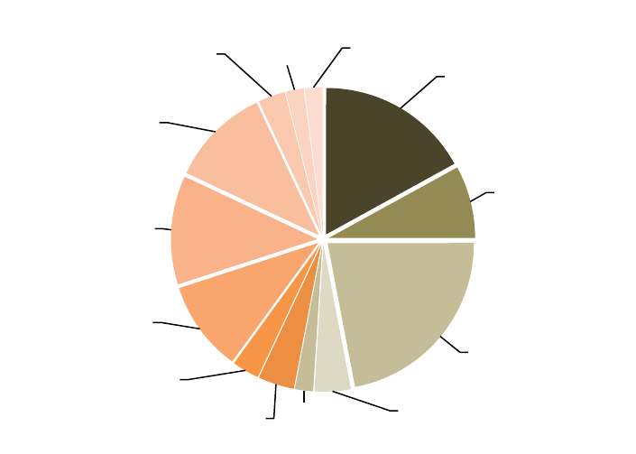
73
3.8 CSP Installation and Operations and Maintenance Cost Trends
The average cost, after federal incentives, for a CSP plant without storage is greater than
$4,000/kW in the United States (Bullard et al. 2008). For example, investment for construction
and associated costs for the 64 MW Nevada Solar One plant amounted to $260 million or about
$4,100/kW (Acciona Energy 2008). System developers strongly believe that improvements in
design will reduce this cost considerably, making it more competitive with traditional electricity
sources.
Figure 3.20 shows a typical cost breakdown for components of a parabolic trough system, with
the solar field comprising approximately 50% of the total installed cost; solar field components
include the receivers, mirrors (reflectors), structural support, drivers, and foundation. Receivers
and mirrors each contribute approximately 10% to the total. The power block, which is not
considered part of the solar field, normally has the highest cost of all the major components,
contributing roughly 20% to the total (Pitz-Paal et al. 2005).
Figure 3.20. Generic parabolic trough CSP cost breakdown
(Pitz-Paal et al. 2005)
3.9 CSP Technology Characteristics and System Performance
Four types of CSP technology are currently under development: parabolic trough technology,
power tower technology, dish-engine technology, and linear Fresnel reflector technology.
3.9.1 Parabolic Trough Technology
Trough technology uses one-axis tracking, has a concentration ratio of 80 (concentration ratio is
calculated by dividing reflector area by focal area), and achieves a maximum temperature of
about 400°C. This relatively low temperature limits potential efficiency gains and is more
susceptible to performance loss when dry cooling is used. Moreover, the relatively low operating
Contigencies
(Indirect)
17%
Storage
8%
Power Block
22%
Others
4%
Land
2%
Foundation
4%
Drivers
3%
Mirrors
10%
Structure
12%
Receiver
11%
Instrumentation
and Controls
3%
Connecting
Cables
2%
Piping of
Headers
2%
74
temperature makes it very difficult to provide the amount of heat storage (in a cost-effective
manner) that is required for around-the-clock dispatchability (Grama et al. 2008, Emerging
Energy Research 2007).
3.9.2 Power Tower Technology
Receiver technology uses two-axis tracking, has a concentration ratio up to 1,500, and achieves a
maximum temperature of about 650°C (Grama et al. 2008). The higher operating temperature of
tower technology reduces susceptibility of these systems to efficiency losses, especially when
dry cooling is used. The reflectors, called heliostats, comprise 40% of capital costs (Emerging
Energy Research 2007).
3.9.3 Dish-Engine Technology
Dish-engine technology uses two-axis tracking, has a concentration ratio up to 1,500, and
achieves a maximum temperature of about 700°C (Emerging Energy Research 2007). This
technology set the world record for solar thermal conversion efficiency, achieving 31.25%
(Andraka 2008).
3.9.4 Linear Fresnel Reflector Technology
Linear Fresnel reflector technology uses one-axis tracking, has a concentration ratio of 80, and
achieves a maximum temperature of about 400°C. The reduced efficiency (15% to 25%)
compared to troughs is expected to be offset by lower capital costs (Grama et al. 2008, Emerging
Energy Research 2007).
3.9.5 Storage
Thermal energy storage (TES) has the potential to extend CSP production time up to 16 hours
per day, increasing capacity factor to more than 50% and allowing for greater dispatchability.
Although capital expenditure increases when storage is added, the LCOE will most likely
decrease because of the increased capacity factor and greater utilization of the power block
(NREL 2009c). Moreover, storage increases the technology’s marketability, as utilities can
dispatch the electricity to meet non-peak demand. For example, a molten salt mixture of 60%
sodium nitrate and 40% potassium nitrate is used as the storage medium for the 50-MW
Andasol I plant located in Spain, enabling more than 7 hours of additional electricity production
after direct-normal insolation is no longer available. Various mixtures of molten salt are being
investigated to optimize the storage capacity, and research is being conducted on other mediums
such as phase-change materials. Synthetic mineral oil, which has been the historical heat transfer
fluid used in CSP systems, is also being viewed as a potential storage medium for future systems.
3.9.6 Heat-Transfer Fluid
Improvements in the heat-transfer fluid (HTF) are necessary to bring down the LCOE for CSP.
This can be accomplished by lowering the melting points and increasing the vapor pressure of
these substances. Dow Chemical’s and Solutia’s synthetic mineral oils have been used widely as
the HTF in trough systems. The problem with these synthetic oils is that they break down at
higher temperatures, preventing the power block from operating at higher, more efficient
temperatures. Molten salts can withstand higher temperatures than the currently available

75
synthetic oils and are being considered as an HTF. The downside is that they freeze at a higher
temperature than the synthetic oils, which means a drop in temperature during the night may
solidify the substance. This, in turn, can damage the equipment when the salt expands and puts
pressure on the receivers. Corrosion of the receivers is another potential concern when salts are
introduced. Nonetheless, research is being conducted to use this substance as both an HTF and
TES medium. If this can be accomplished, costly heat exchangers would not be needed, thus
helping to reduce the LCOE.
3.9.7 Water Use
As stated previously in Section 2.4.4, a water-cooled parabolic trough plant typically requires
approximately 800 gallons per MWh. Power towers operate at a higher temperature and have
lower water cooling needs, ranging from 500–750 gallons per MWh. Dish-engine systems do not
require water cooling. As CSP plants are usually constructed in dry regions, water-scarcity issues
and competing uses are of concern (except for dish-engine systems). An alternative to water
cooling is dry or air cooling, which eliminates about 90% of water consumption (U.S. DOE
2009). However, air cooling requires higher upfront capital costs and can result in a 5% decrease
in electricity generation, depending on location temperature. This plant-efficiency reduction
amounts to a 2%–9% increase in LCOE . An alternative is to implement hybrid cooling, which
decreases water use while minimizing the generation losses experienced with dry cooling.
3.9.8 Land Requirements
The amount of acreage needed for a CSP facility depends partly on the type of technology
deployed. More importantly, though, land use is dependent on thermal storage hours and a
location’s solar insolation. Common practice is to state land requirements in terms of acres per
MW. The range normally provided is 4–8 acres in a location with solar insolation similar to that
found in the U.S. desert Southwest (SNL 2009). The low end of the range is possible when
greater self-shading of reflectors is allowed, although this results in reduced electricity output.
The high end represents the additional land needed for energy storage, with energy storage
resulting in higher capacity factor. Because of such variation, when considering land needs, it
can be more useful to provide a number in terms of acres per MWh. When this is done, a
comparison among CSP technology types can more easily be made. The general trend at this
stage of technology development is that power towers require approximately 20% more land per
MWh than troughs. Commercial dish-engine facilities have not yet been built, so a comparison
of land requirements for this technology with other CSP technologies has not yet been made.
3.10 References
Acciona Energy. (2008). www.acciona-na.com. Accessed November 2008.
Andraka, C. E. (July 2, 2008). Statement of Charles E. Andraka, Sandia National Laboratories.
Concentrating Solar Power. United States Senate Committee on Energy and Natural Resources
Field Hearing in Albuquerque, New Mexico.
Bartlett, J.E.; Margolis, R.M.; Jennings, C.E. (September 2009). The Effects of the Financial
Crisis on Photovoltaics: An Analysis of Changes in Market Forecasts from 2008 to 2009.
National Renewable Energy Laboratory. Technical Report NREL/TP-6A2-46713.
http://www.nrel.gov/docs/fy10osti/46713.pdf. Accessed September 2009.

76
Bullard, N.; Chase. J.; d’Avack, F. (May 20, 2008). “The STEG Revolution Revisited.” Research
Note. London: New Energy Finance.
Canada, S.; Moore, L.; Post, H.; Strachan, J. (2005). "Operation and Maintenance Field
Experience for Off-grid Residential Photovoltaic Systems." Prog. Photovolt: Res. Appl.; 13:67–
74.
Denholm, P.; Margolis, R. (2008a). Supply Curves for Rooftop Solar PV Generated Electricity
for the U.S. NREL Report TP-670-44073. Golden, CO: National Renewable Energy Laboratory.
Denholm, P.; Margolis, R. (2008b). “Impacts of Array Configuration on Land-Use Requirements
for Large-Scale Photovoltaic Deployment in the United States.” NREL Conference Paper
CP-670-42971. Golden, CO: National Renewable Energy Laboratory.
Denholm, P.; Margolis, R. (2008c). “Land-Use Requirements and the Per-Capita Solar Footprint
for Photovoltaic Generation in the United States.” Energy Policy; 36:3531–3543.
Emerging Energy Research, LLC. (2007). Global Concentrated Solar Power Markets and
Strategies, 2007–2020. Cambridge, MA: Emerging Energy Research.
Grama, S.; Wayman, E.; Bradford, T. (2008). Concentrating Solar Power—Technology, Cost,
and Markets. 2008 Industry Report. Cambridge, MA: Prometheus Institute for Sustainable
Development and Greentech Media.
Kazmerski, L. (November 2009). “Best Research-Cell Efficiencies.” Golden, CO: National
Renewable Energy Laboratory.
Knoll, B.; Kreutzmann, A. (April 2008). “Market survey on on-grid inverters 2008.” Photon
International, pp.104–111.
Kreutzmann, A. (February 2008). “Solar modules in 2008.” Photon International, pp.126–135.
Mehos, M.; Kearney, D. (2007). “Potential Carbon Emissions Reductions from Concentrating
Solar Power by 2030.” Kutscher, C. ed. Tackling Climate Change in the U.S.: Potential Carbon
Emissions Reductions from Energy Efficiency and Renewable Energy by 2030. NREL Report
CH-550-41270. Boulder, CO: American Solar Energy Society, pp. 79–89.
www.ases.org/climatechange/
. Accessed June 2009.
Mehta, S.; Bradford, T.; (2009). PV Technology, Production, and Cost, 2009 Forecast: The
Anatomy of a Shakeout. Prometheus Institute and Greentech Media.
Mints, P.; Tomlinson, D. (2006). Photovoltaic Manufacturer Shipments 2005/2006. Report #
NPS-Supply1. Palo Alto, CA: Navigant Consulting Photovoltaic Service Program.
Mints, P.; Tomlinson, D. (2008). Photovoltaic Manufacturer Shipments & Competitive Analysis
2007/2008. Report # NPS-Supply3. Palo Alto, CA: Navigant Consulting Photovoltaic Service
Program.
Mints, P. (2009). Photovoltaic Manufacturer Shipments, Capacity, & Competitive Analysis
2008/2009. Report # NPS-Supply4. Palo Alto, CA: Navigant Consulting Photovoltaic Service
Program.
Moore, L.; Post, H.; Hayden, H.; Canada, S.; Narang, D. (2005). "Photovoltaic Power Plant
Experience at Arizona Public Service: A 5-year Assessment." Prog. Photovolt: Res. Appl.;
online.

77
Moore, L.M.; Post, H.N. (2007). "Five Years of Operating Experience at a Large, Utility-Scale
Photovoltaic Generating Plant." Prog. Photovolt: Res. Appl.; online.
Moore, L.M.; Post, H.N. (2008). "Five Years of Residential Photovoltaic System Experience at
Tucson Electric Power." Strategic Planning for Energy and the Environment; 28:2, pp. 58–73.
NREL. (2009a). LCOE analysis for U.S. cities. Golden, CO: National Renewable Energy
Laboratory (internal only).
NREL. (2009b). PVWatts: A Performance Calculator for Grid-Connected PV Systems.
Version 1. Golden, CO: National Renewable Energy Laboratory.
http://rredc.nrel.gov/solar/codes_algs/PVWATTS/version1/. Accessed August 2009.
NREL. (2009c). Solar Advisor Model (SAM). Version 3.0. Modeling runs conducted for troughs
and towers in July 2009. Golden, CO: National Renewable Energy Laboratory (internal only).
NREL. (2009d). Photovoltaic Solar Resource: United States – Spain – Germany. Produced by
Billy Roberts of the NREL Geographic Information System (GIS) team.
Photon International. (1999–2008). Annual market surveys for solar modules.
Photon International. (2002–2008). Annual market surveys for on-grid inverters.
Pitz-Paal, R.; Dersch, J.; Milow, B., eds. (February 16, 2005). European Concentrated Solar
Thermal Road-Mapping (ECOSTAR). Roadmap Document. European Union: European
Commission. http://www.solarpaces.org/Library/library.htm. Accessed November 20, 2009.
Renewable Energy Policy Network for the 21
st
Century (REN21). (2008). Renewables 2007
Global Status Report 2007. Paris: REN21 Secretariat. www.ren21.net/publications
. Accessed
February 2009.
Sandia National Laboratories (SNL). (September 2009). E-mail correspondence with CSP
technical staff. Albuquerque, NM: Sandia National Laboratories.
U.S. Bureau of Economic Analysis (BEA). (2009). National Income and Product Accounts
(NIPA): GDP Implicit Price Deflator Data. http://www.econstats.com/nipa/NIPA1_1_1_4_.htm.
Published August 20, 2009.
U.S. Department of Energy (DOE). (2009). Report to Congress. Concentrating Solar Power
Commercial Application Study: Reducing Water Consumption of Concentrating Solar Power
Electricity Generation.
www.eere.energy.gov/solar/pdfs/csp_water_study.pdf. Accessed October
2009.
Wiser, R.; Barbose, G.; Peterman, C.; Darghouth, N. (2009). Tracking the Sun II. The Installed
Cost of Photovoltaics in the U.S. from 1998–2008. Berkeley, CA: Lawrence Berkeley National
Laboratory.
http://eetd.lbl.gov/ea/EMS/re-pubs.html. Accessed October 2009.
Wohlgemuth, J.H.; Cunningham, D.W.; Nguyen A.M.; Miller J. (2006). Long Term Reliability of
PV Modules. Frederick, MD: BP Solar.
78
4. Policy and Other Market Drivers
This chapter covers key elements of U.S. federal, state, and local policies pertaining to solar
energy technologies, as well as market-based developments that affect U.S. solar market
evolution. Section 4.1 discusses federal policies, incentives, and programs including tax credits,
depreciation benefits, grants, the DOE loan guarantee program, clean renewable energy bonds,
and other federal programs and incentives. Section 4.2 discusses state and local policies and
incentives, and rules and regulations including permitting, interconnection, net metering, direct
cash incentive programs, renewable portfolio standards and solar set-asides, and clean energy
funds. Section 4.3 provides information on major financing mechanisms and programs: third-
party power purchase agreement financing, customer solar lease financing, property-assessed
clean energy programs, and other emerging financing structures.
4.1. Federal Policies and Incentives, PV and CSP
Federal policies and incentives play an important role in the commercialization and adoption of
solar technologies; they have enabled rapid expansion of solar markets in countries such as
Germany, Spain, and Japan. Legislation enacted in the United States in 2008 and early 2009
provides unprecedented levels of federal support for U.S. renewable energy projects, including
solar energy projects.
The Emergency Economic Stabilization Act of 2008 (EESA or “bailout bill”) became law on
October 3, 2008. It contains tax incentives designed to encourage individuals and businesses to
invest in renewable energy, including 8-year extensions of the business and residential solar
investment tax credits (ITCs).
The American Recovery and Reinvestment Act (ARRA or “stimulus bill”) was signed into law
on February 17, 2009, with an estimated $787 billion overall in tax incentives and spending
programs. Many ARRA provisions support solar energy.
This section discusses the major U.S. federal policies and incentives directed toward solar
energy, with an emphasis on provisions in the EESA and ARRA. For additional information,
including how to apply for the benefits of the policies, see the list of Web sites at the end of this
section.
4.1.1 Investment Tax Credit
Sections 48 (for businesses) and 25D (for residences) of the Internal Revenue Code detail the
federal ITC for certain types of energy projects, including “equipment which uses solar energy to
generate electricity." Like other tax credits, the ITC reduces the tax burden of individuals and
commercial entities that make investments in solar energy technology. On an industry level, a
long-term ITC provides consistent financial support for growth such as building manufacturing
plants, developing an installer workforce, and investing in large-scale solar electric plants that
require extended planning and construction time.
For commercial projects, the ITC is realized in the year in which the solar project begins
commercial operations, but vests linearly over a 5-year period (i.e., one-fifth of the 30% credit
vests each year over a 5-year period). Thus, if the project owner sells the project before the end

79
of the fifth year since the start of commercial operations, the unvested portion of the credit will
be recaptured by the IRS. This period is sometimes referred to as the 5-year “clawback” period.
The EESA extended the ITC through December 31, 2016, including extensions of the
commercial and residential solar ITCs, providing a credit of up to 30% of the total capital costs
of a project (including equipment and labor) (SEIA 2008).
53
4.1.2 Renewable Energy Grants
The EESA removed the cap on the
ITC for residential PV systems (previously $2,000), effective for property placed in service after
December 31, 2008. The bill also allows individual taxpayers to use the credit to offset
alternative minimum tax liability. Another change to the ITC was to allow regulated utilities to
claim the tax credit, providing significant support for increased utility investment in solar energy
projects. The ARRA enhanced the ITC further by allowing individuals and businesses to qualify
for the full amount of the solar tax credit, even if projects receive subsidized energy financing.
Previously, the ITC would not apply to the portion of the investment funded via subsidized
financing such as below-market loans. Also, the ARRA removed the $2,000 cap on the ITC for
residential solar water heating systems.
Section 1603 of the ARRA authorizes the Department of the Treasury to issue renewable energy
project developers cash grants in lieu of the ITC. The grants program was created in response to
the lack of available financing and limited appetite for tax credits resulting from the financial
crisis and economic downturn. The program is designed like the ITC and offers an equivalent
30% benefit based on the cost of the solar property that is placed in service.
Grants are available for qualifying property that is placed in service during 2009 and 2010. Solar
projects that commence construction by December 31, 2010, and are placed in service prior to
2017 also qualify. Developers must apply for the grant by September 30, 2011, and only
taxpaying corporate entities are eligible. Grant applications will be processed within 60 days
from the date it is received or the system is placed in service, whichever is later.
There are several variables that determine whether a developer might opt to apply for a cash
grant. These factors may include state and local incentives and mandates, project scale and
required lead time for development, and the ability to monetize tax credits. The Treasury
Department began accepting applications for grants on July 31, 2009, and the first payments
were announced on September 1. By the end of November 2009, 65 solar projects had received
funds, with allocations totaling more than $18 million.
More information is available online: http://www.treasury.gov/recovery/1603.shtml
53
Historically, through 2005, the size of the commercial solar credit was equal to 10% of the project’s “tax credit basis,” the
portion of system costs to which the ITC applies. The Energy Policy Act of 2005 temporarily increased the solar credit to 30% of
a project’s tax credit basis, for projects placed in service between January 1, 2006, and January 1, 2008. In late December 2006,
the Tax Relief and Healthcare Act of 2006 extended the in-service deadline to December 31, 2008, and in October 2008, the
EESA extended it once again for a full 8 years, through December 31, 2016. Unless extended again or otherwise altered over the
next 8 years, the Section 48 commercial solar credit will revert back to 10% for projects placed in service on January 1, 2017.

80
4.1.3 Manufacturing Tax Credit
The ARRA created a tax credit for new investments in advanced energy manufacturing that,
similar to the ITC, is equal to 30% of the investment. Eligible technologies include renewable
energy, energy conservation, electric grids supporting intermittent sources of renewable energy,
carbon capture and storage, biofuel refining or blending, and hybrid-electric vehicles and
components. The cap for new manufacturing investment credits is $2.3 billion, supporting
$7.7 billion of manufacturing capital investment.
54
In determining which projects receive the tax
credits, the Treasury Department, in coordination with the Department of Energy, will consider
the following factors: commercial viability, job creation, greenhouse gas impact, technological
innovation and cost reduction, and time to completion. More information is available online:
http://www.energy.gov/recovery/48C.htm
4.1.4 MACRS and Bonus Depreciation
Section 168 of the tax code allows investors to depreciate certain investments in solar power
(and other types of) projects using a 5-year accelerated depreciation schedule known as the
Modified Accelerated Cost Recovery System (MACRS). Under this provision, “equipment
which uses solar energy to generate electricity” qualifies for 5-year, double declining-balance
depreciation. In most cases, 100% of a solar project’s cost will qualify for this accelerated
schedule, but the 30% ITC will reduce the project’s depreciable basis by 15%. Assuming a 40%
combined effective state and federal tax bracket and a 10% nominal discount rate, on a present-
value basis, this 5-year MACRS depreciation schedule provides a tax benefit equal to about 26%
of system costs (Bolinger 2009).
55
In addition to the standard MACRS, the EESA includes a bonus depreciation schedule for solar
projects installed in 2008. Qualifying projects can receive 50% depreciation in the first year, with
the remaining 50% depreciated over the 5-year MACRS schedule. The ARRA extends the 50%
year-one bonus depreciation incentive for qualified renewable energy investments made through
2009. The ARRA also extends through 2009 a recent increase in the size of the write-off
available (up to 100% of a $250,000 investment, a declining percentage after $250,000, and
phasing out at $800,000).
Taken together, the 30% ITC and accelerated depreciation
provide a combined tax benefit equal to about 56% of the installed cost of a commercial solar
system (Bolinger 2009).
4.1.5 Renewable Energy Loan Guarantee Program
The DOE loan guarantee program established by Title XVII of the Energy Policy Act of 2005
was expanded by the ARRA to include a new Section 1705 loan guarantee program, in addition
to the existing Section 1703 program. The ARRA permitted the guarantee of about $40 billion of
loans by the Section 1705 program, in addition to the $51 billion authorized for Section 1703.
Table 4.1 summarizes the loan guarantee programs, including differences pertaining to project
eligibility and benefits.
54
Of the $2.3 billion in total awards to 183 projects, more than $1.0 billion went to 60 solar projects. See:
http://www.whitehouse.gov/the-press-office/president-obama-awards-23-billion-new-clean-tech-manufacturing-jobs
55
Only 12% of this benefit is attributable to the acceleration of the depreciation schedule; the remaining 14% would
be realized even if the project were instead depreciated using a less-advantageous, 20-year straight-line schedule.

81
Table 4.1. DOE Loan Guarantee Programs
Year
FY 2007
FY 2008
FY 2009 Omnibus
FY 2009 ARRA
Amount
$4.0 billion
$38.5 billion
$8.5 billion
$40 billion (estimated)
Authorization
EPACT 2005, Title XVII, Section 1703
EPACT Section 1705,
added by ARRA
Uses
New or significantly improved technologies
Commercial and novel
technologies
Credit Subsidy
Borrower pays
$4.0 billion appropriated
Term
Available until used
Projects must be started by
September 30, 2011
Carve-outs
No carve-out
stipulated by
Congress
• $10.0 billion for
energy efficiency,
renewable energy, and
advanced transmission
and distribution
technologies
• $18.5 billion for
advanced nuclear
power facilities
• $2.0 billion for “front
end” nuclear fuel cycle
facilities
• $6.0 billion for coal-
based power
generation, industrial
gasification, and
carbon capture and
sequestration
• $2.0 billion for
advanced coal
gasification
The FY 2009
Omnibus Budget
provides an
additional
$8.5 billion in loan
authority for
energy efficiency,
renewable energy,
and advanced
transmission and
distribution
projects
No carve-outs were
stipulated, but three project
categories were listed:
• Renewable energy
installations and
manufacturing facilities
for renewable energy
components
• Electric power
transmission systems
• Advanced biofuel
projects
U.S. DOE 2009c
Projects eligible for the Section 1703 program include those that “avoid, reduce or sequester air
pollutants or anthropogenic emissions of greenhouse gases; and employ new or significantly
improved technologies as compared to commercial technologies,” including energy efficiency,
renewable energy, and advanced transmission and distribution as well as advanced nuclear
power, advanced coal-based power, and carbon capture and sequestration technologies.
Section 1705 is limited to renewable energy installations and manufacturing facilities for
renewable energy components, electric power transmission systems, and advanced biofuel
projects and is targeted toward projects at the commercialization stage (though new or earlier
stage technologies are still eligible). The Section 1705 program requires projects to commence
construction by September 30, 2011, encouraging near-term deployment. Another difference is
that the Section 1705 program provides for DOE to pay the cost of credit subsidies, required up-
front payments equal to about 10% of a loan guarantee's value, up to a total of $4 billion.
56
There are currently two open solicitations, released by DOE in July 2009. The first solicitation is
for "new or significantly improved" energy efficiency, renewable energy, and advanced
transmission and distribution technologies. It combined the authorities of the Section 1703 and
56
The FY 2009 ARRA appropriation for the credit subsidy was originally $6 billion; however, $2 billion were
transferred to the Car Allowance Rebate System (also known as the "Cash for Clunkers" program).

82
1705 programs; projects eligible for 1703 but not 1705 may still secure a loan guarantee, but
may not receive 1705 appropriations to cover the credit subsidy cost. The $2.5 billion in
1705 appropriations allocated to this solicitation include $2 billion for renewable energy and
transmission projects and $0.5 billion for advanced biofuels.
The second solicitation is for large transmission infrastructure projects using commercial
technologies. The authority for the second solicitation is only under Section 1705, so all projects
under this solicitation must commence construction by September 30, 2011. The second
solicitation was allocated $750 million from Section 1705 appropriations to cover the credit
subsidy fees. Combined, these two solicitations are estimated to result in about $30 billion in
loan guarantees.
The first of several loan guarantees was conditionally awarded on March 20, 2009, under the
1703 solicitation and closed on September 4, 2009, in the amount of $535 million, for Solyndra,
Inc., based in Freemont, California. The funds will support the construction of a manufacturing
plant for its proprietary cylindrical solar PV panels, which are expected to provide systems with
low installed cost and high solar electricity output (U.S. DOE 2009d).
For more information on DOE loan guarantee program solicitations, see
http://www.lgprogram.energy.gov/keydocs.html
.
4.1.6 Clean Renewable Energy Bonds
Clean renewable energy bonds (CREBs) were established by EPACT 2005 to provide renewable
project financing for non-taxable entities (governmental entities, electric cooperatives, and public
power providers) that cannot directly use the ITC for solar facilities, production tax credits for
other types of renewable energy facilities, or accelerated tax-depreciation benefits. CREBs are
“tax credit bonds,” which means that the bond purchaser receives a federal income tax credit in
lieu of interest payments. From the borrower’s perspective, CREBs are essentially the equivalent
of a zero-interest loan, aside from the various transaction costs of bond issuance described
below, which reportedly can be considerable (Cory et al. 2008).
The CREB program received an initial allocation of $800 million in 2005 (round 1), which was
then increased to $1.2 billion by legislation in 2006, providing a second allocation of about
$400 million (round 2). The round 1 CREB allocation of $800 million was awarded in 2006. The
round 2 CREB allocation of $477 million was awarded in 2008 (the extra $77 million was due to
surrendered volume from the first allocation). Of the $1.2 billion CREB allocations, state and
local governments were limited to $750 million or 62.5% of allocations, with the rest intended
for municipal and cooperative electric companies (DSIRE 2010a).
The Energy Improvement and Extension Act of 2008 authorized $800 million and the ARRA
authorized an additional $1.6 billion for new CREBs, for a total allocation of $2.4 billion
(round 3). In April 2009, the IRS opened a solicitation for the $2.4 billion allocation, which
closed on August 4, 2009. In October 2009, $2.2 billion of CREBs applications were given
issuing authority by the IRS for a period of 3 years. Round 3 CREBS funding was to be allocated
as follows: one-third for qualifying projects of state/local/tribal governments, one-third for
public power providers, and one-third for electric cooperatives (DSIRE 2010a).

83
Figure 4.1. Distribution of round 1 and 2 CREB
allocation, percent of projects by technology
(IRS 2006, IRS 2007)
Figure 4.2. Distribution of round 3 CREB
allocation, percent of projects by technology
(IRS 2009)
Figures 4.1 and 4.2 capture the distribution of CREB allocations by technology. By number of
projects, solar accounted for 62% of round 1 and 2 (year 2006-2008) allocations and 89% of
round 3 (2009) allocations (IRS 2006, IRS 2007, IRS 2009).
57
By funding amount, solar
accounted for 21% or $84 million of round 2 allocations and 38% or $839 million of round 3
allocations (IRS 2007, IRS 2009).
58
4.1.7 Solar on Federal Property
The EESA and ARRA together appropriated $5.5 billion to the Federal Buildings Fund for green
building improvements including energy efficiency measures and the use of renewable energy
sources such as solar. Of the total appropriation, $4.5 billion will be available to federal facilities
managed by the General Services Administration (Cory et al. 2009, Prometheus 2009).
4.1.8 State Energy Program
Funding from DOE’s State Energy Program (SEP) goes to state energy offices in all states and
U.S. territories. Under ARRA, SEP will distribute $3.1 billion to the states (U.S. DOE 2009e).
Activities eligible for SEP funding include energy audits, building retrofits, education and
training efforts, and new financing mechanisms to promote renewable energy investments. Many
of the state governments will use part of these funds to support solar programs and installations.
For every dollar of federal investment in SEP, the states estimate saving $7.22 in energy costs
and also leveraging $10 of non-federal investment in energy projects, typically by cosponsoring
energy projects with local and private partners (U.S. DOE 2009e). For more information on the
DOE State Energy Program, see: http://apps1.eere.energy.gov/state_energy_program/.
57
The percentages for round 2 are based on data representing $405 million in initial funding for round 2.
58
Detailed funding amounts for round 1 are not available. The percentages for round 2 are based on data
representing $405 million in initial funding for round 2.
Solar
62%
Wind
23%
Landfill
Gas
8.8%
Biomass
2.8%
Hydro-
power
2.6%
Other
< 1%
Solar
89%
Wind
5.9%
Biomass
1.9%
Hydro-
power
3.2%
Other
< 1%

84
4.1.9 Energy Efficiency and Conservation Block Grant Program
The Energy Efficiency and Conservation Block Grants (EECBG) Program, authorized in the
Energy Independence and Security Act of 2007, was funded for the first time by the ARRA
(DOE 2009a). Through formula
59
and competitive grants, the U.S. DOE will distribute
$3.2 billion to U.S. cities, counties, states, territories, and Indian tribes to develop, implement,
and manage energy efficiency and conservation projects and programs (U.S. DOE 2009b). Local
and state governments may utilize funds for solar installations on government buildings and
engage in energy strategy development, which may include solar energy technology, along with
energy efficiency and conservation. For more information on the DOE EECBG, see:
www.eecbg.energy.gov.
4.1.10 Renewable Energy Production Incentive
The Renewable Energy Production Incentive (REPI), a federal incentive for renewable energy
systems, was implemented as part of the Energy Policy Act (EPACT) of 1992 and amended in
EPACT 2005 to expand eligible facilities and authorize federal appropriations through 2026.
Qualified facilities are categorized as Tier 1 (solar, wind, ocean, geothermal, closed-loop
biomass) and Tier 2 (open-loop biomass such as landfill gas and livestock methane; municipal
solid waste is excluded). The program originated to support facilities owned by public utilities
and other nonprofit load-serving entities (LSEs), providing per kWh-based payments for the first
10 years of operation. The actual payment amount is dependent on availability of federal budget
appropriations each year (U.S. DOE 2008). Historically, the REPI program has been
insufficiently funded and has not made full payments for the electricity generated by qualifying
facilities since 1995.
60
4.1.11 Additional Resources
With continued uncertainty over the funding appropriation from year to
year, the REPI program is likely to serve only as a supplementary incentive program.
For additional information, including how to apply for the benefits of the policies, see the
following Web sites:
• DOE Solar Energy Technologies Program Financial Opportunities
(www.eere.energy.gov/solar/financial_opportunities.html)
•
DOE Energy Efficiency & Renewable Energy (EERE) Financial Opportunities
(www.eere.energy.gov/financing/)
• DOE EERE Recovery Act Web site (www.eere.energy.gov/recovery/)
• U.S. Department of the Treasury, American Recovery and Reinvestment Act
(www.treasury.gov/recovery)
59
More information on the formula methodology for EECBG can be found at:
http://www.eecbg.energy.gov/downloads/EECBG_Federal_Register_Notice_04_15_09.pdf.
60
For production year 2007, DOE paid out only $2.7 million of the $11.25 million in eligible funds to Tier 1
projects and $1.8 million of the nearly $8 million in eligible funds to Tier 2 projects (U.S. DOE 2008). Only a small
fraction of these funds have gone to solar projects; the average payment was about $900 for each of the 25 solar
projects in 2007 (Cory et al. 2008).

85
• U.S. Internal Revenue Service (IRS), Energy Provisions of the American Recovery and
Reinvestment Act of 2009 (www.irs.gov/newsroom/article/0,,id=206871,00.html)
• Solar Energy Industries Association (SEIA), Government Affairs & Advocacy
(www.seia.org/cs/government_affairs_and_advocacy)
• Database of State Incentives for Renewables & Efficiency (www.dsireusa.org)
4.2 State and Local Policies, Incentives, and Rules and Regulations
As outlined in the previous section, there are a number of federal-level financial incentives
available to support the increased deployment of solar energy technologies. State and local
policies work in parallel with these federal-level initiatives, but go beyond financial incentives to
include renewable energy mandates and other mechanisms to further stimulate adoption of solar
energy technologies. State legislators and utility commissioners hold primary responsibility for
setting a state’s overarching energy policy and regulatory framework. How solar technologies
are treated in this process will significantly affect how, or even if, a solar market develops in a
state. Local governments also influence solar policies. In areas where the local government has
jurisdiction over a utility, the government can directly influence solar rebate programs and
renewable generation requirements. In areas served by investor-owned utilities or cooperatives,
local governments can still play an important role in solar market development by streamlining
permitting processes or developing innovative financing mechanisms.
State and local policies in support of increased solar deployment are more prevalent than federal
policies and have a well-established history of both successes and failures. As such, states and
regions with stronger and longer-term policies and incentives, coupled with a favorable
electricity market (e.g., higher than average electricity prices) and an adequate solar resource,
have established pockets of wide-scale solar installations. In addition, because states are often
innovation hubs, there is a continuous flow of new policies and approaches to driving solar
development that bears watching.
4.2.1 Planning and Permitting
Planning is an effort by governments to ensure community land and resources are used in a
beneficial manner. Permits are allowances issued by governments to ensure that activities
undertaken within their jurisdictions meet established guidelines. Planning and permitting are
important steps in the installation of solar technologies. Done properly, they ensure that a solar
project meets necessary safety, operational, environmental, and community compatibility
standards while not unduly hindering the project's completion. However, planning and permitting
processes not well designed for solar applications can increase the cost and time requirements of
a project substantially or even create enough delay and difficulty that the project is not
completed.
Section 2.4.5 describes some of the planning and permitting issues related to utility-scale solar
installations. This section focuses on planning and permitting by local and state governments for
smaller-scale, distributed PV installations. Installing a grid-connected PV system requires an
electrical permit from the local government and, in some cases, a building permit followed by
inspection of the installation (DOE 2009f).
86
Numerous planning and permitting barriers can hinder distributed PV system installation. The
following have been identified as most significant (Pitt 2008):
• Complex and unclear local permitting requirements
• Inspectors and permitting authorities inexperienced with renewable energy systems
• Permitting requirements that vary significantly across jurisdictions
• Permit fees that are high enough to become a significant, additional project cost
• Unfair and often illegal enforcement of restrictive housing covenants.
Recommendations to local and state governments for overcoming planning and permitting
barriers include the following (Pitt 2008, U.S. DOE 2009f):
• Understand the entire permitting and inspection process for PV systems and the dynamics
between all entities involved.
• Establish a clear path for communication between code enforcement offices and the local
utility provider to expedite the interconnection and inspection processes.
• Remove barriers to PV systems from building and zoning codes.
• Simplify PV permit application forms and review processes.
• Allow over-the-counter building permits for standard roof-mounted systems that do not
exceed the roof support capabilities of a structure meeting minimum building code
requirements.
• Adopt flat permit fees or fee waivers for PV systems.
• Ease permitting processes by establishing statewide interconnection standards (see
Section 4.2.2 below) and educating building and electrical inspectors about proper
installation procedures for distributed renewable energy systems.
• Adopt state-level legislation mandating consistent and appropriate permitting
requirements for distributed renewable energy systems.
A number of U.S. cities have led the way in modifying their planning and permitting policies to
encourage solar energy development (U.S. DOE 2009f). For example, San Jose, California,
grants electrical permits for PV systems over the counter and requires building permits only for
rooftop installations that meet certain criteria. Portland, Oregon, allows residential PV installers
to submit permit applications online and trains some permitting staff to be experts on solar
installations. Madison, Wisconsin, amended city laws to comply with state statutes that make it
illegal to forbid PV systems in historic districts. The Solar America Board for Codes and
Standards released a model expedited permitting process in October 2009 (Brooks 2009).
Continued efforts such as these will be necessary to expedite implementation of PV systems in
communities nationwide.
4.2.2 Interconnection
Interconnection standards specify the technical, legal, and procedural requirements by which
customers and utilities must abide when a customer wishes to connect a PV system to the grid
(or electricity distribution system). State governments can authorize or require their state public
utility commissions to develop comprehensive interconnection standards. Some state
interconnection standards apply to all types of utilities (investor-owned utilities, municipal

87
utilities, and electric cooperatives); other states have chosen to specify standards only for
investor-owned utilities. Although most utilities fall under the jurisdiction of state public utility
commissions, cities with municipal utilities can have significant influence over interconnection
standards in their territory.
The aspects of interconnection standards that are most often debated are procedural, not
technical, in nature. In setting technical interconnection standards, most regulatory bodies
reference compliance with the Institute of Electrical and Electronics Engineers’ (IEEE’s) “1547
Standard for Interconnecting Distributed Resources with Electric Power Systems,” which was
adopted in 2003. The most debated procedural aspects of interconnection standards are:
requirements for small inverter-based PV systems to have a utility external disconnect switch
(UEDS), limitations placed on PV system size, technical screens for interconnection, and
requirements for additional insurance (NNEC 2009).
States continue to demonstrate a mix of approaches to these key aspects. Eight states and many
major utility companies have recognized that safety devices and features already built into all
code-compliant PV systems make the UEDS redundant in small systems (less than 10 kW) and
have eliminated its requirement (Sheehan 2008).
61
Many states leave the UEDS requirement to
utility discretion. Interconnection standards with regard to PV system-size limitations also vary
widely among states, ranging from 10 kW to no cap on system size. As of November 2009,
seven states
62
and Puerto Rico specify no limit on system size (DSIRE 2009). The size of the PV
system and complexity of the interconnection typically dictate the rigor and extent of the
technical screens required before interconnection.
States also differ in their approaches to the issue of insurance requirements. States and some
utilities require owners of solar PV systems that are interconnecting to the grid to purchase
additional liability insurance to mitigate the risks of potential personal injury (e.g., to utility workers)
and property damage (NNEC 2009).
Thirteen states plus Washington, D.C., and Puerto Rico
require varying levels of insurance based on system size (IREC 2009).
63
Other states, including
Arizona, Indiana, Iowa, New Mexico, and Washington, leave the insurance requirement to utility
discretion (IREC 2009). Twelve states
64
do not require additional insurance and seven states
65
Figure 4.3 shows that 37 states plus Washington, D.C., and Puerto Rico have adopted an
interconnection policy. All of the states with robust solar markets have interconnection policies
in place. Robust solar markets do not exist in any of the states without interconnection policies.
do
not specify insurance as part of their interconnection standards (IREC 2009).
61
The eight states that have waived the UEDS requirement for small systems are Arkansas, Delaware, Florida,
Nevada, New Jersey, New Hampshire, North Carolina, and Utah. Utilities that have waived the UEDS requirement
for small systems include Pacific Gas and Electric (PG&E) and Sacramento Municipal Utility District (SMUD) in
California and National Grid U.S.A. in the Northeast United States.
62
California, Hawaii, Indiana, New Hampshire, North Carolina, Michigan, and Vermont do not have limits on the
capacity of interconnected solar PV systems (DSIRE 2009).
63
States with insurance requirements based on the size of the interconnected system are Colorado, Connecticut,
Delaware, Florida, Illinois, Massachusetts, Michigan, Minnesota, Missouri, Oregon, South Dakota, Virginia, and
Wisconsin.
64
States that do not require additional insurance for interconnected solar PV systems are California, Georgia,
Hawaii, Kentucky, Nevada, New Hampshire, New Jersey, New York, North Carolina, Pennsylvania, South
Carolina, and Vermont.
65
States that have not specified insurance requirements as part of their interconnection standards are Arkansas,
Louisiana, Maryland, Montana, Ohio, Texas, and Wyoming.
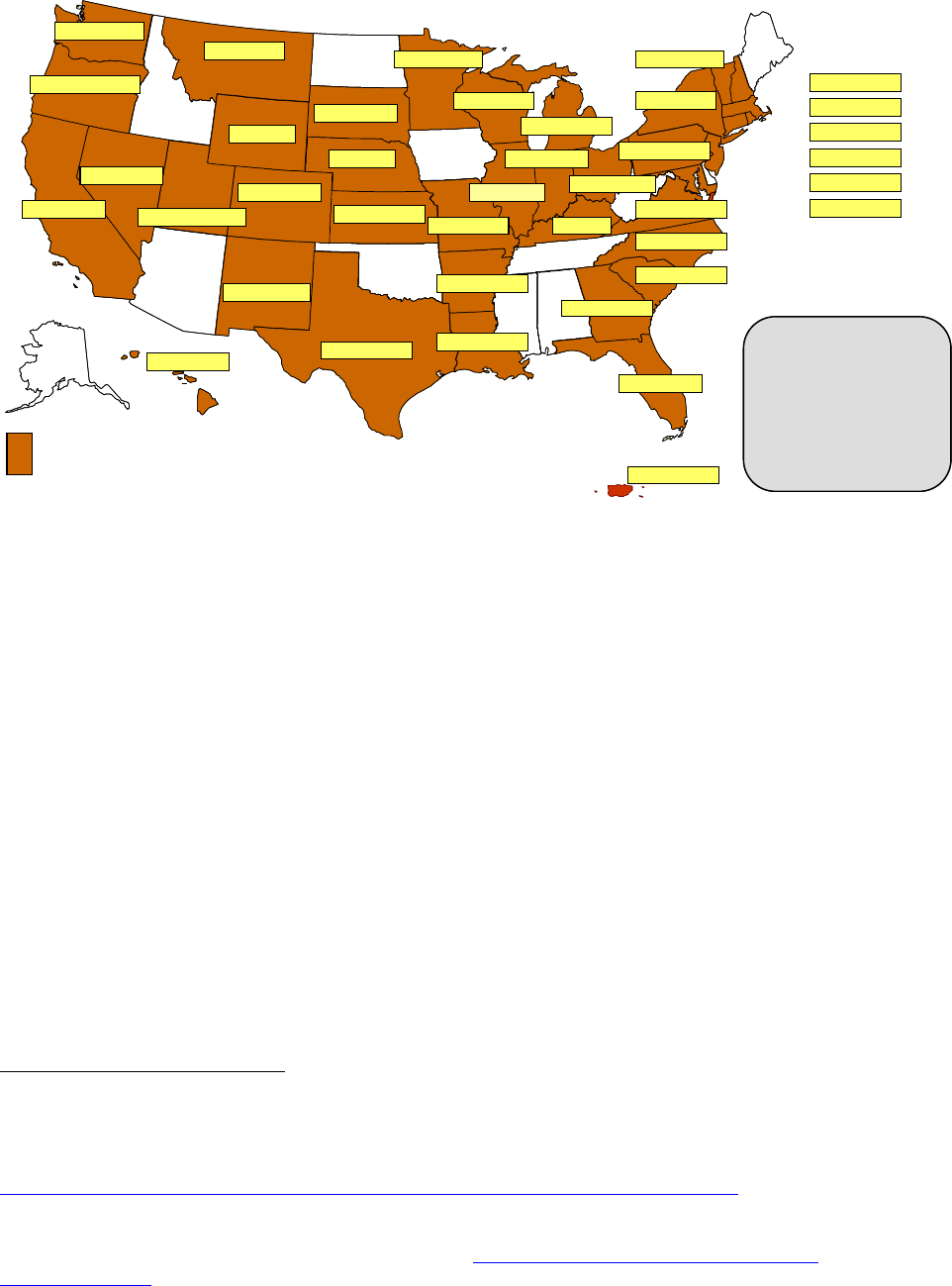
88
Figure 4.3. Interconnection Standards, November 2009
66
(DSIRE 2010b)
In the absence of a national interconnection standard, state regulators often consider the four
leading interconnection models when developing such policies.
67
These models include the
Federal Energy Regulatory Commission’s Small Generator Interconnection Procedure (SGIP)
and Small Generator Interconnection Agreement, California Rule 21, the Mid-Atlantic Demand
Resource Initiative’s Model Interconnection Procedures, and the Interstate Renewable Energy
Council’s (IREC’s) Model Interconnection Standards for Small Generator Facilities.
68
All four
procedures have comprehensive coverage of interconnection standards including specifications
for interconnecting systems up to 10 MW, pro forma interconnection agreements, fast-track
procedures for systems up to 2 MW, and a review process for interconnecting larger systems
(typically greater than 10kW).
69
California Rule 21, which was approved in December 2000 and
updated slightly based on utility tariff filings, is used for the interconnection of all solar and
distributed generation (DG) systems in utility service territories in California, which constitute a
majority of the solar installations in the United States (Keyes and Fox 2008).
66
Numbers for each state indicate system capacity limits in kW. Some state limits vary by utility, customer type
(e.g., residential/non-residential), technology, and/or system application. “No limit” means that there is no stated
maximum size for individual systems. Generally, state interconnection standards apply only to investor-owned
utilities. For more detail on the interconnection standards for each state, see
http://www.dsireusa.org/incentives/index.cfm?SearchType=Interconnection&&EE=0&RE=1.
67
U.S. Representative Jay Inslee (D-Washington) introduced the Clean Energy Buy-Back Act in March 2008, which
included federal interconnection standards. The bill did not pass.
68
For more details on the four interconnection models, see: www.solarabcs.org/interconnection/ABCS-
07_studyreport.pdf.
69
IREC and SGIP have simplified interconnection procedures for systems of 10 kW or less; California Rule 21
prequalifies systems less than 11 kW for three of the eight necessary technical screens (Keyes and Fox 2008).
State policy
*
Standard only applies to net-metered systems
WA: 20,000
OR: 10,000
CA: no limit
MT: 50*
NV: 20,000
UT: 25/2,000*
NM: 80,000
WY: 25*
HI: no limit
CO: 10,000
MN: 10,000
LA: 25/300*
AR: 25/300*
MI: no limit
WI: 15,000
MO: 100*
IN: no limit
IL: 10,000
FL: 2,000*
KY: 30*
OH: 20,000
NC: no limit
VT: no limit
NH: 100*
MA: no limit
37 states +
DC & PR
have adopted an
interconnection
policy
CT: 20,000
PA: 5,000*
NJ: 2,000*
DC: 10,000
MD: 10,000
NY: 2,000
VA: 20,000
SC: 20/100
GA: 10/100*
PR: no limit
TX: 10,000
NE: 25*
KS: 25/200*
SD: 10,000
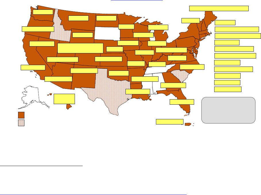
89
4.2.3 Net Metering
Net metering is a policy that allows PV system owners to offset electricity purchases from the
utility with every kilowatt-hour of solar electricity a PV system produces. As with
interconnection standards, state governments can authorize or require their state public utilities
commissions to develop comprehensive net metering rules, and cities with municipal utilities can
have significant influence over net metering rules in their territory.
Net metering is one of the most important policy drivers for distributed PV systems because it
enables system owners to recover some of their investment through electricity bill savings
(Coughlin and Cory 2009). Under the simplest implementation of net metering, a utility
customer’s billing meter runs backward as solar electricity is generated and exported to the
electricity grid and runs forward as electricity is consumed from the grid. At the end of a billing
period, a utility customer receives a bill for the net electricity, which is the amount of electricity
consumed less the amount of electricity produced and exported by the customer’s PV system.
Figure 4.4 illustrates the variety of net-metering, system-size limitations across the United States.
Currently, 42 states and Washington, D.C., have net metering policies in place. Net metering
policies differ in several ways, including the eligibility of different technology types, customer
classes, system sizes, the use of aggregate caps for DG contribution back to the grid, the
treatment of customer net-excess generation, the types of affected utilities, and the issue of REC
ownership (IREC and NCSC 2007). Detailed state-specific information regarding net-metering
availability and regulation is available through the Web site for the Database of State Incentives
for Renewables & Efficiency (DSIRE) (www.dsireusa.org/
).
Figure 4.4. Net Metering Policies, October 2009
70
(DSIRE 2009)
70
Numbers for each state indicate system capacity limits in kW. Some state limits vary by utility, customer type
(e.g., residential/non-residential), technology, and/or system application. “No limit” means that there is no stated
maximum size for individual systems. For more detail on the net metering standards for each state, see
http://www.dsireusa.org/incentives/index.cfm?SearchType=Net&&EE=0&RE=1.
RI: 1,650/2,250/3,500*
MA: 60/1,000/2,000*
PA: 50/3,000/5,000*
State policy
Voluntary utility program(s) only
*
State policy applies to certain utility types only (e.g., investor-owned utilities)
WA: 100
MT: 50*
NV: 1,000*
UT: 25/2,000*
AZ: no limit*
ND: 100*
NM: 80,000*
WY: 25*
HI: 100
KIUC: 50
CO: no limit
co-ops & munis: 10/25
OK: 100*
MN: 40
LA: 25/300
AR: 25/300
MI: 150*
WI: 20*
MO: 100
IA: 500*
IN: 10*
IL: 40*
FL: 2,000*
KY: 30*
OH: no limit*
GA: 10/100
WV: 25
NC: 1,000*
VT: 250
VA: 20/500*
NH: 100
CT: 2,000*
NY: 25/500/2,000*
NJ: 2,000*
DE: 25/500/2,000*
MD: 2,000
DC: 1,000
42 states + DC
have adopted a
net metering policy
NE: 25
KS: 25/200*
ME: 660, co-ops & munis: 100
PR: 25/1,000
OR: 25/2,000*
CA: 1,000*
90
4.2.4 Direct Cash Incentive Programs
Direct cash incentives give solar energy system owners cash back for a qualified solar
installation. Qualified solar installations vary by state and may include solar electricity-
producing, water heating, and space heating and cooling technologies. Direct cash incentives
include rebates, grants, and production- or performance-based incentives that complement other
financial incentives such as tax credits.
The manner and timing in which direct cash incentives are paid varies by location and program
design. Rebate and grant amounts are often based on system size or system cost, and the funding
is typically awarded at the time of installation. Performance or production-based incentives are
distributed to project owners over several years based on the amount of energy the system
produces. Expected performance rebates are based on solar system capacity as well as system
rating, location, tilt and orientation, and shading. Expected performance rebates may be
distributed in a lump sum, but are calculated based on the expected energy output of the system.
Payments based on performance or expected performance instead of capital investments are
gaining prominence among program administrators because they encourage optimized system
design and installation. To avoid a boom-and-bust cycle that can disrupt solar energy markets,
careful consideration should be given to incentive levels, program caps, and long-term funding
mechanisms for direct cash incentive programs.
California, the leading U.S. state in terms of installed PV capacity, provides an example of a
direct cash incentive program. In January 2006, the California Public Utilities Commission
launched the California Solar Initiative (CSI), a direct cash incentive program providing more
than $3 billion for solar energy projects with the objective of installing 3,000 MW of solar
capacity by 2016. CSI includes a transition to performance-based and expected performance-
based incentives (as opposed to up-front payments based only on system size), with the aim of
maximizing system performance through effective system design and installation. CSI incentive
levels will automatically be reduced over the duration of the program in ten steps based on the
aggregate capacity of solar installed in each utility service area. The California Public Utility
Commission designated funding sources for the CSI program for 10 years (2006–2016).
Figure 4.5 shows the states in which direct cash incentives are available.
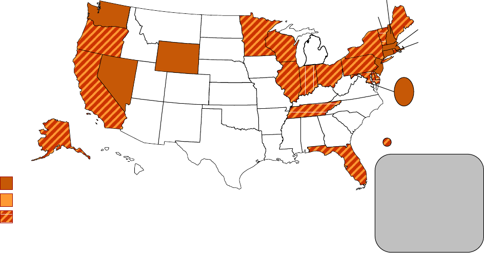
91
Figure 4.5. States that offer direct cash incentives for solar projects, September 2009
(DSIRE 2009)
States and utilities usually administer direct cash incentive programs, but some local
governments also offer these incentives to consumers. Currently, approximately 24 states and
more than 100 utilities offer direct incentives for solar installations. Direct cash incentives are
often funded through a public or systems benefits fund, clean energy funds, a revolving loan
fund, or the general fund. The incentives typically cover 20% to 50% of project costs and range
from a few hundred to millions of dollars (U.S. DOE 2009f).
4.2.5 Renewable Portfolio Standards and Solar Set-Asides
A renewable portfolio standard (RPS) is a policy that requires utilities or load-serving entities
(LSEs) to provide its customers with a certain amount of electricity generated from renewable
resources. While an RPS is typically a mandate, it can also be a non-binding goal; it is almost
always stated as a percentage of the total electricity provided to be reached by a predetermined
future date (Bird and Lockey 2008). As indicated in Figure 4.6, 29 states plus the District of
Columbia have renewable portfolio standards in place, and an additional 6 states have non-
binding renewable energy production goals.
U
State Direct Cash Incentives for PV
State Direct Cash Incentives for Solar Water Heating
State Direct Cash Incentives for both PV and Solar Water Heating
DC
24 States +
DC and the
Virgin Islands
offer Direct Cash
Incentives for
Solar Projects
U
U
U
U
U
U
U
U
U
U
U
U
U
U
U
UU
U
U
U
U
U
U
U
U
U
VT
NH
MA
RI
U
U
Utility Direct Cash Incentive(s) for PV and/or Solar Water Heating
U.S. Virgin Islands
U
U
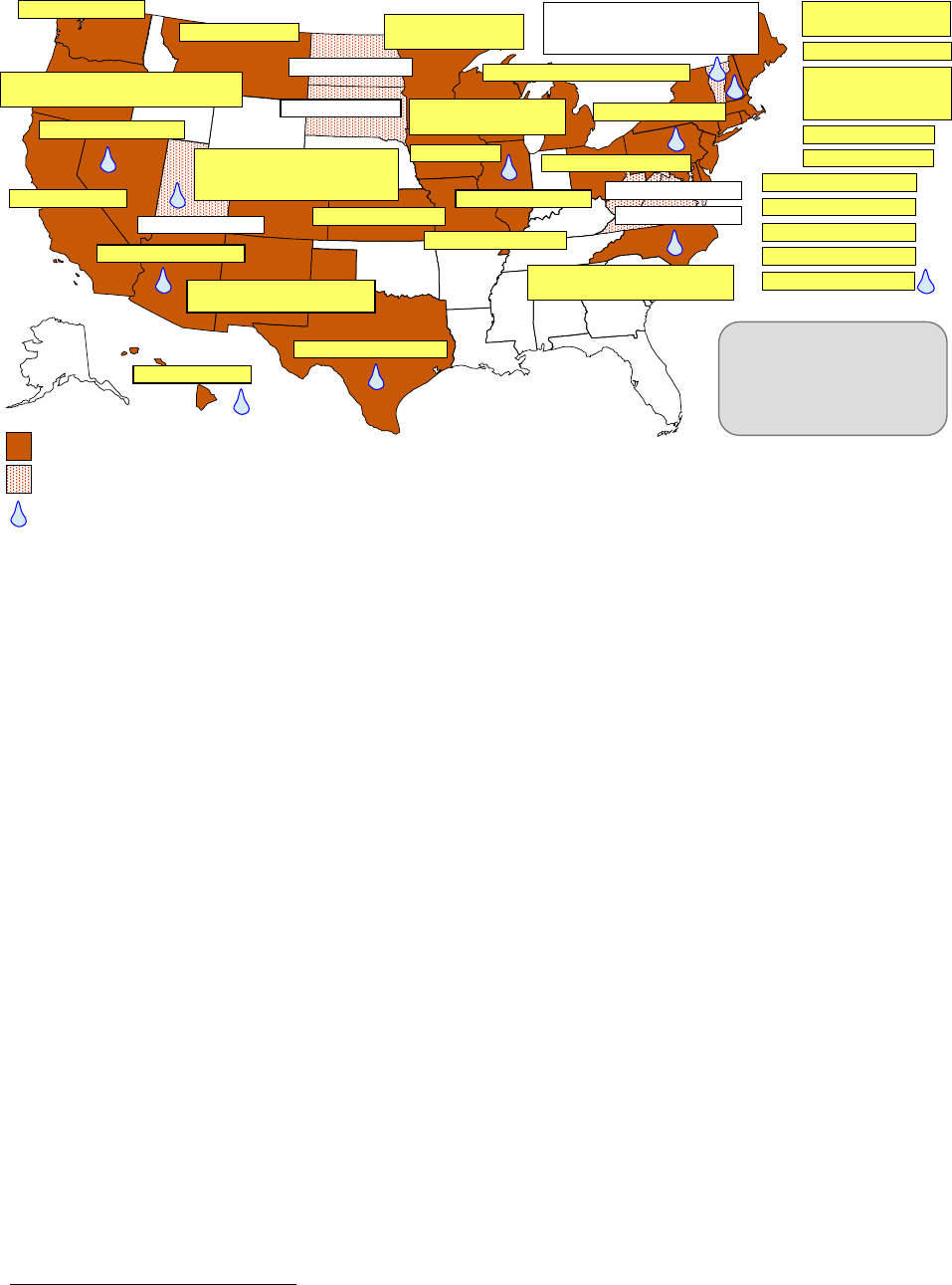
92
Figure 4.6. State renewable portfolio standards and goals, October 2009
(DSIRE 2009)
In effect, two products are produced from renewable energy generation: the environmental
attributes sold in the form of renewable energy credits (RECs) and the actual electricity produced
by the renewable generator. A REC typically represents the attributes of 1 MWh of electricity
generated from renewable energy. An unbundled REC represents the environmental benefits
without the actual energy, and bundled RECs include both the environmental benefits and the
actual energy produced by a renewable source. Many states allow RECs to be bought unbundled
from the associated electricity and used to fulfill RPS obligations (Holt and Wiser 2007).
A growing number of states are incorporating a “set-aside” or “carve-out” within the RPS,
stipulating that a portion of the required renewable energy percentage or overall retail sales be
derived from solar or DG resources
71
71
Note that when solar PV is located on residential, business, or government property and not part of a large
centralized power system, it is considered to be distributed generation.
(DSIRE 2009). Figure 4.7 shows 15 states along with
Washington, D.C., that have these set-asides or carve-outs for solar electricity generation and
solar water heating. In addition, Massachusetts legislation has established a DG set-aside, but
specific targets have not yet been established. Only three states and Washington, D.C., allow
solar water heating to count toward the solar set-aside requirements. Figure 4.7 illustrates that
solar electricity demand based on existing RPS set-aside requirements alone would amount to the
installation of more than 8 GW of cumulative installed solar capacity by 2025 (Wiser and
Barbose 2008, Wiser and Barbose 2009).
State renewable portfolio standard
State renewable portfolio goal
Solar water heating eligible
*
†
Extra credit for solar or customer-sited renewables
Includes non-renewable alternative resources
WA: 15% by 2020*
☼ NV: 25% by 2025*
☼ AZ: 15% by 2025
☼ NM: 20% by 2020 (IOUs)
10% by 2020 (co-ops)
HI: 40% by 2030
☼
Minimum solar or customer-sited requirement
TX: 5,880 MW by 2015
UT: 20% by 2025*
☼ CO: 20% by 2020 (IOUs)
10% by 2020 (co-ops & large
munis)*
MT: 15% by 2015
ND: 10% by 2015
SD: 10% by 2015
IA: 105 MW
MN: 25% by 2025
(Xcel: 30% by 2020)
☼ MO: 15% by 2021
WI: Varies by utility;
10% by 2015 goal
MI: 10% + 1,100 MW by 2015*
☼ OH: 25% by 2025†
ME: 30% by 2000
New RE: 10% by 2017
☼ NH: 23.8% by 2025
☼ MA: 15% by 2020
+ 1% annual increase
(Class I Renewables)
RI: 16% by 2020
CT: 23% by 2020
☼ NY: 24% by 2013
☼ NJ: 22.5% by 2021
☼ PA: 18% by 2020†
☼ MD: 20% by 2022
☼ DE: 20% by 2019*
☼ DC: 20% by 2020
VA: 15% by 2025*
☼ NC: 12.5% by 2021 (IOUs)
10% by 2018 (co-ops & munis)
VT: (1) RE meets any increase in
retail sales by 2012;
(2) 20% RE & CHP by 2017
29 states + DC
have an RPS
6 states have goals
KS: 20% by 2020
☼ OR: 25% by 2025 (large utilities)*
5% - 10% by 2025 (smaller utilities)
☼ IL: 25% by 2025
WV: 25% by 2025*†
CA: 33% by 2020
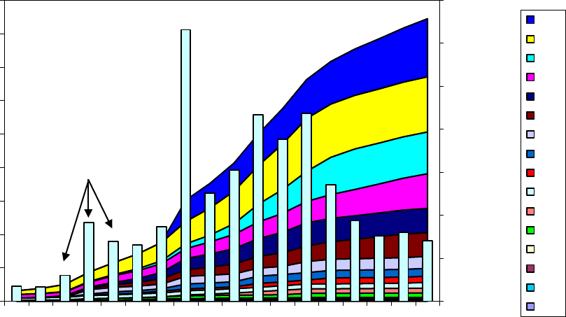
93
Figure 4.7. Solar capacity to meet existing RPS solar set-aside requirements, November 2009
(Wiser and Barbose 2009)
As with the overall RPS requirements, to reach the goal of the solar set-aside, utilities or LSEs
can either own the solar generation capacity or purchase bundled or unbundled solar RECs
(SRECs) (Cory et al. 2008). One major difference between RECs and SRECs is their cost;
SRECs typically generate more revenue than RECs, providing an additional financial incentive
to install solar power systems. To create a value for RECs and SRECs, however, the RPS must
include a penalty or alternative compliance mechanism that has a distinctly higher penalty for
those not complying with the RPS or solar set-aside (Cory and Coughlin 2009).
SRECs are one of the key elements that can make a third-party PV ownership project financially
feasible, resulting in as much as 40% to 80% of revenues for third-party PV projects. Two states
that have witnessed high revenues from SRECs are Colorado and New Jersey (where SREC
prices have ranged from $160/MWh to $265/MWh). In New Jersey, SREC prices are expected to
rise from $300/MWh to $711/MWh in 2009 as the up-front rebates are removed (Cory et al.
2008).
New Jersey announced its Solar Renewable Energy Credit Registration Program in August 2009,
designed to incentivize solar development in the state. One SREC is issued for each MWh of
electricity generated from a solar electric system. The SRECs represent all the clean energy
benefits from the solar generation and are sold or traded separately from the power, providing
solar system owners with a source of revenue to help offset the costs of installation. The New
Jersey SREC Program is expected to almost entirely replace the state’s rebates, which fueled
solar growth in the early years of the state’s solar program.
0
200
400
600
800
1,000
1,200
1,400
0
1,000
2,000
3,000
4,000
5,000
6,000
7,000
8,000
9,000
2008
2009
2010
2011
2012
2013
2014
2015
2016
2017
2018
2019
2020
2021
2022
2023
2024
2025
Annual Solar Additions (MW)
Cumulative Solar Capacity (MW)
IL
NJ
MD
AZ
PA
OH
NM
NC
MO
NV
DE
CO
DC
NH
OR
NY
Annual Capacity
(right axis)
Cumulative
Capacity
(left axis)
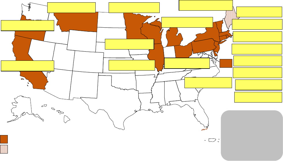
94
4.2.6 Clean Energy Funds
In the mid- to late-1990s, a bevy of states introduced retail competition and with it concerns over
continued funding for energy efficiency, renewable energy, and low-income energy assistance
programs. To address those concerns, system (or public) benefit funds were established and
supported through an additional charge to end-users’ electricity bills, either as a per-kWh charge
or a flat fee. The fund is then dispersed in various forms, such as grants, loans, and rebates, to
support investments in renewable energy, energy efficiency, and related improvements for low-
income housing. Eligibility to receive support from a system benefit fund is contingent on the
recipient being an electricity ratepayer (Cory et al. 2008).
As Figure 4.8 indicates, the systems benefits charges can amount to large funds in the aggregate.
For example, California is expecting to raise more than $4 billion from 1998 to 2016, and New
Jersey expects to raise $647 million from 2001 to 2012. Across the nation, an estimated
$7.3 billion in 16 states and Washington, D.C., will have been collected by 2017.
In subsequent years, a second generation of “clean energy funds” was created and supported
through a variety of methods, including RPS alternative compliance payments, general fund
obligations, and oil and gas severance tax payments. These clean energy funds typically support
energy efficiency and renewable energy programs and represent a renewed interest by states in
the deployment of clean energy technologies. These second-generation funds were established in
Alaska, Colorado, Iowa, and Maryland.
Figure 4.8. Estimated system benefit funds for renewables, May 2009
(DSIRE 2009)
The way in which these funds are dispersed varies from state to state. In California, for example,
the system benefit fund supports the CSI outlined in Section 4.2.3.
State PBF supported by voluntary contributions
* Fund does not have a specified
expiration date
** The Oregon Energy Trust is scheduled
to expire in 2025
RI: $2.2M in 2009
$38M from 1997-2017*
MA: $25M in FY2009
$524M from 1998-2017*
NJ: $78.3M in FY2009
$647M from 2001-2012
DE: $3.4M in 2009
$48M from 1999-2017*
CT: $28M in FY2009
$444M from 2000-2017*
VT: $5.2M in FY2009
$33M from 2004-2011
PA: $950,000 in 2009
$63M from 1999-2010
IL: $3.3M in FY2009
$97M from 1998-2015
NY: $15.7M in FY2009
$114M from 1999-2011
WI: $7.9M in 2009
$90M from 2001-2017*
MN: $19.5M in 2009
$327M from 1999-2017*
MT: $750,000 in 2009
$14M from 1999-2017*
OH: $3.2M in 2009
$63M from 2001-2010
MI: $6.7M in FY2009
$27M from 2001-2017*
ME: 2009 funding TBD
$580,300 from 2002-2009
DC: $2M in FY2009
$8.8M from 2004-2012
DC
OR: $13.8M in 2009
$191M from 2001-2017**
CA: $363.7M in 2009
$4,566M from 1998-2016
State PBF
16 states + DC
have public benefits
funds ($7.3 billion
collected by 2017).
ME has a voluntary
public benefits fund
95
It is important to note that the state funds have been instrumental in driving the installation of
grid-connected PV systems; more than 75% of the grid-connected PV systems installed in the
United States in 2007 were located in states with a clean energy fund. Moreover, the state funds
have invested more than 75% of their available funding in PV projects (Clean Energy States
Alliance 2009).
4.2.7 Emerging Trends
Several policy/financing mechanisms are emerging that have the potential to incite further solar
market expansion through the establishment of widespread local and utility programs. The three
topics discussed in this section are feed-in tariffs, property tax financing, and rate structures.
A feed-in tariff (FIT) is a requirement for utilities to purchase electricity from eligible renewable
systems at a guaranteed price over a fixed period. Alternatively, a FIT can consist of a fixed or
variable premium above the market price. A FIT increases the rate of PV deployment by
providing a more stable revenue stream from PV systems and improving the rate of return on PV
investments. The payment level generally is designed to ensure that the systems are able to
recover costs and provide a modest profit. In addition to offering guaranteed prices, FITs
typically guarantee grid access, allowing both small and large projects to connect to the grid
according to uniform interconnection standards. FITs have been used extensively in Europe and
are starting to be implemented in the United States (Couture and Cory 2009).
Municipalities and counties across the country are launching innovative public/private financing
programs that allow property owners to spread the cost of renewable energy systems over the
long term. For example, Berkeley, California, and Boulder, Colorado, have passed initiatives to
allow homeowners and businesses the opportunity to finance PV systems through adjustments to
their property taxes, thus taking advantage of the government entities’ tax-free financing
capabilities to support expansion of these resources at the local level. Programs utilizing this
financing approach are commonly referred to as property-assessed clean energy (PACE)
programs and will be discussed in more detail in Section 4.3.3, along with other innovative
financing mechanisms.
As customer-sited generation and advanced metering technologies become more prevalent, there
is an increased interest in developing alternative rate structures that reflect the resulting changes
in electricity use. The majority of existing rate structures do not capture the actual value of time-
varying increases or decreases in demand for electricity, and therefore are unlikely to capture the
value of energy produced by customer-sited generation including solar PV. This is because solar
PV peak generation often correlates well with peak electricity demand. With the availability of
more advanced metering, it is possible to create rate structures that better reflect the variances in
the value of electricity as demand fluctuates. Appropriate rate structures for PV could enable
better capture of the value of excess customer generation exported to the grid. While time-of-use
rates and other emerging rate structures are still relatively uncommon, it is anticipated that they
will become increasingly more prevalent and serve as a driver for solar market expansion.
96
4.3 Private Sector and Market-Based Developments to Facilitate Solar
Deployment
The financing of solar and other renewable energy technologies experienced significant changes
in 2008 and early 2009. The passage of the ARRA in February 2009 greatly expanded the
availability and usability of various tax credits, depreciation opportunities, loan guarantees, and
other mechanisms designed to incent private and public investment in renewable energy and
energy efficiency projects. The ARRA expanded and extended an array of incentives made
available with passage of the EESA (and other earlier laws).
In addition to the previously described support mechanisms, private sector and other solar market
stakeholders, including states, counties, and municipalities, have developed mechanisms to
support renewable energy financing by residents, businesses, and institutional and government
consumers of energy.
Three prominent financing mechanisms/programs for solar PV and CSP will be discussed in this
section: the third-party power purchase agreement (PPA), the solar lease, and property-assessed
clean energy (PACE) programs.
4.3.1 Third-Party Power Purchase Agreement Financing
All sectors can use the third-party ownership PPA, including homeowners, businesses, utilities,
and state and local governments.
In a third-party ownership PPA model, one party hosts a PV system on his or her property and a
solar developer purchases, installs, owns, operates, and maintains the system. In the residential
sector, it is the homeowner that hosts and does not purchase or own the PV system, and instead
buys the electricity produced by the PV system under a long-term PPA (see Figure 4.9). In
exchange for signing the PPA, the homeowner avoids paying for the PV system up front and
usually is not responsible for the operation and maintenance (O&M) of the system. The PPA
provider receives the monthly cash flows in the form of power sales and the fully monetized
federal tax benefits, including the investment tax credit and accelerated depreciation. An
example of a PPA provider for the residential (and commercial) market is SolarCity, which
offers a variety of lease structures, including a zero-down option; however, the higher the down
payment, the lower the monthly lease payment (Coughlin and Cory 2009).
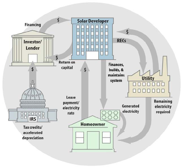
97
Figure 4.9. The residential power purchase agreement
(NREL 2009b)
The commercial PV market has witnessed a rapid proliferation of the use of the PPA-financing
model of ownership. Greentech Media estimated that roughly 80% of the commercial market in
2008 will have used a PPA for PV installations, an increase from previous levels of 50% in 2007
and 10% in 2006 (Guice and King 2008). The benefits of the PPA method for financing PV
deployment in the commercial sector are similar to those for customers in the residential sectors.
Thus, a PPA provides the opportunity for a commercial owner to host rather than own a PV
system. Instead of securing capital up front and being responsible for O&M, the business owner
signs a long-term PPA to purchase the electricity generated by the system. The PPA is typically
priced at or below the prevailing utility retail rate in the first year (with perhaps some escalation
over the life of the contract). The owner of the business avoids most, if not all, of the up-front
purchase and installation costs, as well as O&M responsibilities.
Utilities often rely on third parties to design, finance, manage construction of, and operate and
maintain solar facilities. Development of these facilities requires the long-term procurement of
the power output. Accordingly, utilities sign PPAs with the developers, allowing the developer to
obtain lower-cost financing, passing on the savings through relatively lower power prices. PPAs
can come in many forms and durations, but generally payments are made for both the plant
capacity (maximum capable output) and energy production, and PPAs cover a 15- to 20-year
period starting with a facility’s commercial operation. However, now that utilities can use the
ITC directly, their use of third-party PPAs may be affected (see Section 4.3.5).
Utilities benefit from PPAs as they are designed to leverage the technical expertise and
experience of the solar developer. PPAs also allocate risks of cost overruns, plant availability,
etc., to a pre-specified party, typically the plant developer. In return for accepting most

98
development and operating risks, the developer receives price certainty and marketability of its
product.
PPAs allow faster development of solar resources as utilities can leverage the capability of many
developers simultaneously. For example, Pacific Gas & Electric has approximately 3 GW of
large-scale CSP and PV solar facilities under development via its PPA counterparties, including
such entities as BrightSource Energy, First Solar, Sun Power, Solel, and Solaren Corp.
(Mendelsohn and Kreycik, forthcoming).
State and local governments are also responding to the challenges of funding PV development on
their buildings and land by using innovative finance structures such as the third-party-ownership
PPA model. As with the residential and commercial sectors, the benefits of transferring the up-
front costs and O&M responsibilities to the owner/developer, maintaining steady electricity
prices, and using federal tax benefits inherent to the PPA ownership model have made it an
attractive option for state and local properties.
Note that third-party PPA financing may face regulatory or legal challenges in some states,
especially where the issue of utility commission regulation of third-party owned systems has not
been specifically addressed (Kollins, forthcoming).
4.3.2 Customer Solar Lease Financing
The customer solar lease is similar to the residential or commercial PPA in that a property owner
hosts, but does not own, a solar PV system. To take advantage of federal tax incentives, a third-
party lessor finances and owns the solar PV installation. However, distinct to a solar lease, the
property owner (as lessee) pays to use the equipment instead of purchasing the generated power.
Thus, the customer’s lease payment remains constant even if the system’s output fluctuates. If
the system does not meet the customer’s entire energy needs, the customer purchases additional
electricity from his/her utility. Any excess electricity generated by the system can be net
metered, earning the customer cents/kWh credits on his/her electric utility bill.
Similar to a third-party PPA, the solar lease transfers the high up-front costs to the system
owner/developer, who can take advantage of valuable federal tax incentives. Some of the cost
savings might be passed down to the customer in the form of lower payments. In states with
complementary incentives, lease payments can be less than or equal to monthly utility savings.
72
Also, like the third-party PPA, the lease may shift maintenance responsibilities to the developer.
There are challenges associated with the solar lease. For example, the leasing company may not
have as strong an incentive to maintain the system as it would under a third-party PPA contract,
because the customer’s payments are fixed regardless of the system’s output. However, some
companies will monitor the system’s output and will provide maintenance promptly, or will
include a performance guarantee that ensures a minimum kWh output (Kollins et al.,
forthcoming). Also, as with the third-party PPA, the solar lease may face regulatory challenges
in some states (Kollins et al., forthcoming). In addition, the traditional solar lease may not be
available to non-taxable entities such as state and local governments because of uncertainty
72
For lease payments to nearly equal utility bill savings, the leasing company must have additional incentives, such
as up-front rebates or performance based payments (Coughlin and Cory 2009).

99
about renewing contracts on a year-to-year basis. However, state and local governments may be
able to use a tax-exempt lease where payments to the lessor are tax exempt (Bolinger 2009).
4.3.3 Property-Assessed Clean Energy Programs
In addition to private-sector financing mechanisms, local governments have also designed
programs to fund energy efficiency and renewable energy development on private property, with
a particular focus on funding PV installations.
Several municipalities are assisting residential and commercial ownership of renewable energy
systems through financing via property tax assessments.
73
Property-assessed clean energy (PACE) assessments
Piloted by the Berkeley FIRST
program and replicated elsewhere, the property tax assessment model finances the cost of
renewable energy and energy efficiency improvements through the creation of special tax
districts (Coughlin and Cory 2009). Interested property owners may opt into the program and
pay for an additional line item on their property tax bill.
74
transform the high upfront costs into the
equivalent of a moderate monthly payment
75
and allow the property owner to transfer the
assessment and capital improvement to new property owners in the event of a sale (Koenig and
Speer, forthcoming).
76
Figure 4.10 indicates active PACE programs in the United States, as well as states with current
or pending PACE-enabling legislation.
Under a PACE program, a municipality provides the financing to pay for
the up-front system costs for a renewable energy system through an additional property tax
assessment. The municipality funds the assessments by public bond offerings, micro bonds,
general funds, or municipal waste funds (Koenig and Speer, forthcoming). The property owner
repays the cost of the system, plus interest and administrative fees, through additional
assessments placed on his or her property tax bill, which are collected over a time period that
reflects the useful life of the improvements. The property tax assessment model eliminates nearly
all of the up-front costs of installation to the property owner with the exception of program
administrative fees. Further, the renewable energy system and accompanying special property
tax is fixed to the property and not the property owner. Thus, homeowners pay for benefits from
the renewable energy system only while they own the property (Coughlin and Cory 2009;
Koenig and Speer, forthcoming).
73
To date, only the Sonoma County (CA) program is open to commercial property owners. However, Boulder
County (CO) will be opening up the ClimateSmart Loan program to business owners in 2010 with a new round of
funding.
74
Assessments are similar to loans in that they allow a property owner to pay off debt in installments over a long
period of time. However, PACE assessments are not legally considered to be loans.
75
Note that payments are typically made semi-annually. However, the semi-annual payment could be considered by
the property owner as six moderate monthly installments.
76
While property owners may be able to transfer the assessment to a new buyer, a buyer could require that all liens
on the property (including the PACE assessment) be settled before the property is transferred.

100
Figure 4.10. Property-assessed clean energy programs, November 2009
(DSIRE 2010b)
4.3.4 Alternative Financing Structures: Partnership Flips and Leases
PPAs, solar leases, and SRECs are used between a customer and a developer to help finance
solar project development. There are also several other financing mechanisms that are used
between a project developer and a separate tax investor. These financing alternatives are
designed to facilitate full and efficient use of federal and state tax benefits by transferring tax
subsidies to tax-burdened investors. Examples of these financing structures include partnership
flips and leases.
In a partnership flip, ownership of a solar project is shared between a developer and a tax equity
investor, who contributes project investment capital in exchange for federal and state tax benefits
and some revenue. Once the tax equity investor reaches a specified rate of return, the project’s
economic returns are redistributed, or “flipped,” between the developer and tax equity investor,
with the developer typically receiving the majority of electricity sales revenue (Martin 2009).
Solar developers and investors have also financed solar projects with various forms of equipment
leases such as a sale-leaseback and an inverted pass-through. In a sale-leaseback, a developer
sells a solar system and accompanying tax benefits to a tax equity investor, who in turn leases
back the use and possession of the solar property to the same developer (Martin 2009). In an
inverted pass-through lease, the roles of the developer and tax equity investor are effectively
reversed (inverted). The developer makes an election to pass through the investment tax credit to
the tax equity investor along with revenue from the system’s electricity sales. The developer
PACE enabling legislation
Existing authority without new legislation
Active PACE Program
1. Babylon, NY
2. Berkeley, CA
3. Boulder County, CO
4. Palm Desert, CA
5. Sonoma County, CA
1
3
4
5
2
#

101
receives fixed lease payments from the tax equity investor, as well as the tax benefit of
accelerated depreciation (Jones and Lowman 2009).
4.3.5 Increasing Utility Ownership of Solar Projects
Recent federal legislation has also greatly increased the incentive for utilities to directly own
solar projects themselves and not require a separate tax investor. In particular, the EESA
contained three provisions that promote direct utility ownership of solar projects. First, the
8-year investment tax credit extension provides long-term certainty regarding the availability of
the credit. Second, utilities are permitted to take the investment tax credit directly, which was
previously unavailable.
77
Third, the investment tax credit can also be applied to a renewable
energy system owner’s alternative minimum tax―formerly a significant barrier to entry
(Schwabe et al. 2009).
The ARRA also provided an extension of the 50% bonus depreciation in year one in addition to
MACRS, the five-year accelerated depreciation. However, public utilities may not be able to use
MACRS unless their regulators allow them to include the solar property under a normalization
method of accounting (SEPA 2009). Also, utility ownership enables utilities to count electricity
generated toward state RPS requirements.
4.4 References
Bird, L; Lockey, E. (2008). Interaction of Compliance and Voluntary Renewable Energy
Markets. National Renewable Energy Laboratory. NREL Report No. TP-670-42096.
Bolinger, M. (2009). Financing Non-Residential Photovoltaic Projects: Options and
Implications. LBNL Report No. LBNL-1410E. Berkeley, CA: Lawrence Berkeley National
Laboratory.
Brooks, B. (2009). Expedited Permit Process for PV Systems. A Standardized Process for the
Review of Small-Scale PV Systems. Solar America Board for Codes and Standards Report.
http://www.solarabcs.org/permitting/
. Accessed November 2009.
Clean Energy States Alliance. (2009). State Clean Energy Fund Support for Renewable Energy
Projects. Key Findings from the CESA National Database.
www.cleanenergystates.org.
Accessed October 20, 2009.
Cory, K.; Coggeshall, C. Coughlin, J., Kreycik, C. (2009). Solar Photovoltaic Financing:
Deployment by Federal Government Agencies. NREL/TP-6A2-46397. Golden, CO: National
Renewable Energy Laboratory.
Cory, K.; Coughlin, J.; Coggeshall, C. (2008). Solar Photovoltaic Financing: Deployment on
Public Property by State and Local Governments. NREL/TP-670-43115. Golden, CO: National
Renewable Energy Laboratory.
Coughlin, J.; Cory, K. (2009). Solar Photovoltaic Financing: Residential Sector Deployment.
National Renewable Energy Laboratory. NREL/TP-6A2-44853. Golden, CO: National
Renewable Energy Laboratory.
77
Some questions remain about how a utility can take advantage of the ITC under Normalization Accounting rules
(where IOUs have to share tax benefits with customers over time). This is explained further in a forthcoming article,
“Navigating Regulated Investment in Solar Generation: Rewards, Challenges, and Options,” by Alvarez, P., and
Hodges, B., in Electric Perspectives, the magazine of the Edison Electric Institute.

102
Couture, T.; Cory, K. (2009). State Clean Energy Policies Analysis (SCEPA) Project: An
Analysis of Renewable Energy Feed-in Tariffs in the United States. National Renewable Energy
Laboratory. NREL Report No. TP-6A2-45551.
DSIRE. (2009). “Database of State Incentives for Renewables and Efficiency.” Summary Maps.
www.dsireusa.org/summarymaps/index.cfm?ee=1&RE=1. Accessed October 2009.
DSIRE. (2010a). “Database of State Incentives for Renewables and Efficiency.” Clean
Renewable Energy Bonds.
http://www.dsireusa.org/incentives/incentive.cfm?Incentive_Code=US45F&re=1&ee=1.
Accessed January 2010.
DSIRE. (2010b). “Database of State Incentives for Renewables and Efficiency.” Summary
Maps. www.dsireusa.org/summarymaps/index.cfm?ee=1&RE=1. Accessed January 2010.
Guice, J.; King, J.D.H. (February 14, 2008). Solar Power Services: How PPAs are Changing the
PV Value Chain. Prometheus Institute and Greentech Media.
Holt, E.; Wiser, R.H. (2007). The Treatment of Renewable Energy Certificates, Emissions
Allowances, and Green Power Programs in State Renewables Portfolio Standards. Berkeley,
CA: Lawrence Berkeley National Laboratory.
Interstate Renewable Energy Council (IREC); North Carolina Solar Center (NCSC). (2007).
Connecting to the Grid 5th Edition, A Guide to Distributed Generation Interconnection Issues.
www.irecusa.org/fileadmin/user_upload/ConnectDocs/IC_Guide.pdf. Accessed March 16, 2009.
Interstate Renewable Energy Council (IREC). (2008). Updates and Trends.
www.irecusa.org/fileadmin/user_upload/NationalOutreachDocs/IREC_Solar_Market_Trends_Re
vision_11_19_08-1.pdf . Accessed November 16, 2009.
Interstate Renewable Energy Council (IREC). (2009). “State-by-State Interconnection Table.”
http://irecusa.org/wp-content/uploads/2009/11/November_2009_IC_Table.doc. Accessed
December 22, 2009.
Jones, L.; Lowman, D. (2009). “Treasury Grant Program.” Webinar. Hunton and Williams, LLP.
www.hunton.com/media/webinars/recordings/20090714/20090714.html?utm_source=MagnetMa
il&utm_medium=email&utm_term=g[email protected]&utm_content=Treasury%20Grant%20
Program%20Web%20Conference%20Recording%20Available&utm_campaign=martech_0499_
treasury_grant_prgrm_followup_7.15.09. Accessed September 22, 2009.
Kassakhian, Ken. (2009). Clean renewable energy bonds analysis. Golden, CO: National
Renewable Energy Laboratory (internal only).
Koenig, R.; Speer, B. Property Assessed Clean Energy (PACE) Financing: Challenges and
benefits of attracting larger capital investors. Golden, CO: National Renewable Energy
Laboratory (forthcoming NREL technical report).
Kollins, K.; Speer, B.; Cory, K. Solar Photovoltaic Financing: Regulatory and Legal Issues with
Third-Party PPA System Owners. Golden, CO: National Renewable Energy Laboratory
(forthcoming NREL technical report).
Martin, K. (2009). Utility Solar Tax Manual: A Utility Guide to the Federal Investment Tax
Credit. Solar Electric Power Association.

103
Mendelsohn, M.; Kreycik, C. Concentrating Solar Power and Utility Scale Photovoltaics in the
U.S.: Policy Drivers and Financing Incentives. Golden, CO: National Renewable Energy
Laboratory (forthcoming NREL technical report).
Network for New Energy Choices (NNEC) (2009). Freeing the Grid: 2009 Edition. New York, NY:
Network for New Energy Choices.
http://www.newenergychoices.org/uploads/FreeingTheGrid2009.pdf
. Accessed January 18, 2010.
NREL. (2009a). Solar Leasing for Residential Photovoltaic Systems. Fact Sheet. NREL Report
TP-670-43572. Golden, CO: National Renewable Energy Laboratory.
NREL. (2009b). “The residential power purchase agreement.” Golden, CO: National Renewable
Energy Laboratory (internal only).
Pitt, D. (2008). Taking the Red Tape Out of Green Power: How to Overcome Permitting
Obstacles to Small-Scale Distributed Renewable Energy. Network for New Energy Choices.
www.newenergychoices.org/uploads/redTape-rep.pdf. Accessed November 30, 2009.
Prometheus Institute (2009). “Renewable Energy Industry Note.”
www.prometheus.org/system/files/Solar+for+Federal+Buildings.pdf. Accessed December 31,
2009.
Schwabe, P.; Cory, K.; Newcomb, J. (2009). Renewable Energy Project Financing: Impacts of
the Financial Crisis and Federal Legislation. NREL Report No. TP-6A2-44930. Golden, CO:
National Renewable Energy Laboratory.
SEIA. (2008). “The Solar Investment Tax Credit Frequently Asked Questions.” Solar Energy
Industries Association.
http://seia.org/galleries/pdf/ITC_Frequently_Asked_Questions_10_9_08.pdf. Accessed
November 2008.
SEPA. (2009). Utility Solar Tax Manual. Report #02-09. Solar Electric Power Association.
http://www.solarelectricpower.org/resources/reports.aspx. Accessed January 2010.
Sheehan, M. (2008). Utility External Disconnect Switch Practical, Legal, and Technical Reasons
to Eliminate the Requirement. Solar America Board for Codes and Standards.
http://www.solarabcs.org/utilitydisconnect/. Accessed November 20, 2009.
U.S. DOE. (2008). Renewable Energy Production Incentive. U.S. Department of Energy. Office
of Energy Efficiency and Renewable Energy.
http://apps.eere.energy.gov/repi/. Accessed
October 30, 2008.
U.S. DOE. (2009a). Energy Efficiency and Conservation Block Grant Web site. U.S. Department
of Energy. Office of Energy Efficiency and Renewable Energy.
www.eecbg.energy.gov.
Accessed August 2009.
U.S. DOE. (2009b). Energy Efficiency and Conservation Block Grant Program Fact Sheet. U.S.
Department of Energy. Office of Energy Efficiency and Renewable Energy.
www.eecbg.energy.gov/downloads/WIP_EECBG_Fact_Sheet_FINAL_Web.pdf. Accessed
September 2009.
U.S. DOE (2009c). “DOE Loan Guarantee Programs.” U.S. Department of Energy. Solar
Technologies Program and Loan Guarantee Program (internal only).

104
U.S. DOE. (2009d). (March 20, 2009). “Obama Administration Offers $535 Million Loan
Guarantee to Solyndra, Inc.” Press Release. U.S. Department of Energy. Loan Guarantee
Program. www.lgprogram.energy.gov/press/032009.pdf. Accessed September 2009.
U.S. DOE. (2009e). State Energy Program Fact Sheet. U.S. Department of Energy. State Energy
Program. http://apps.eere.energy.gov/state_energy_program/pdfs/sep_factsheet.pdf. Accessed
September 2009.
U.S. DOE. (2009f). Solar Powering Your Community: A Guide for Local Governments. U.S.
Department of Energy. Solar Energy Technologies Program.
www.solaramericacities.energy.gov/resources. Accessed October 2009.
U.S. Department of Treasury, Internal Revenue Service (IRS). (2006). “Clean Renewable Energy
Bond Volume Cap Allocation Information.”
http://www.irs.gov/newsroom/article/0,,id=164423,00.html. Accessed January 2010.
U.S. Department of Treasury, Internal Revenue Service (IRS). (2007). “2007 Disclosure of
Allocations.” http://www.irs.gov/pub/irs-tege/creb_2007_disclosure.pdf. Accessed January 2010.
U.S. Department of Treasury, Internal Revenue Service (IRS). (2009). “New Clean Renewable
Energy Bonds - 2009 Allocations.” http://www.irs.gov/pub/irs-
tege/ncrebs_2009_allocations_v1.1.pdf. Accessed January 2010.
Wiser, R.; Barbose, G. (2008). Renewables Portfolio Standards in the United States. A Status
Report with Data Through 2007. Berkeley, CA: Lawrence Berkeley National Laboratory. LBNL
Report No. LBNL-154E.
Wiser, R.; Barbose, G. (November 2009). “Solar capacity to meet existing RPS solar set-aside
requirements.” Berkeley, CA: Lawrence Berkeley National Laboratory (internal only).

105
5. Investments and Future Outlook
This chapter provides information on trends in private investment in solar energy (Section 5.1), a
summary of DOE investment in solar energy and its role in the solar industry (Section 5.2), and a
review of near-term forecasts for PV and CSP (Section 5.3).
5.1 Private Investment in Solar Energy
This section discusses private investment in solar energy including venture capital (VC), private
equity (PE), debt, public equity, and mergers and acquisitions (M&A) (New Energy Finance
2009).
78
Figure 5.1 shows the tremendous rise of global investment in solar energy, particularly from
2004 to 2008. Total annual investment from 2000 through 2003 was $66 million, $144 million,
$110 million, and $417 million, sequentially, for a 3-year CAGR of 85%. This investment set the
foundation for the rapid expansion of the industry in 2004, as generous incentive programs in
Germany and Japan brought solar energy into the mainstream in both countries. Total investment
in 2005 of $2.5 billion marked a 256% increase over the $702 million of investment in 2004.
This was followed by increases of 183% to $7.08 billion in 2006, 75% to $12.38 billion in 2007,
and 31% to $16.20 billion in 2008.
Private investment in solar energy grew rapidly from 2000 to 2008, with explosive
growth occurring in the latter half of this period. From 2004 to 2008, global private-sector
investment in solar energy increased by a factor of 25 plus. Moreover, the growth in investment
has been widespread, occurring across sources, technologies, and regions. Each of the three
major sources of new investment examined here, venture capital and private equity, debt, and
public equity, grew at a compound annual growth rate (CAGR) of more than 67% from 2004 to
2008. In addition, funding to solar companies increased dramatically for different technologies,
including crystalline silicon PV, thin-film PV, and CPV, and in each of the three main regions,
the United States, European Union, and Asia.
78
An NREL report summarizing private investment information through 2007 was published by NREL in 2008, but
the analysis included in this section was updated by John Bartlett in 2009. The earlier report is: Jennings, C.E.;
Margolis, R.M.; Bartlett, J.E. (2008). Historical Analysis of Investment in Solar Energy Technologies (2000-2007).
National Renewable Energy Laboratory.
www.nrel.gov/docs/fy09osti/43602.pdf.
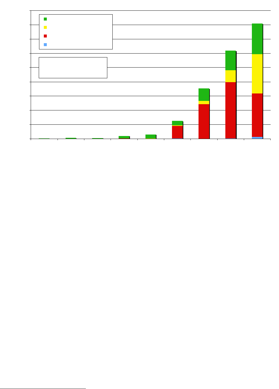
106
Figure 5.1. Global capital investments in solar energy
79
(New Energy Finance 2009)
The role of debt in the solar industry, which totaled $104 million in 2005, $479 million in 2006,
$1.63 billion in 2007, and $5.48 billion in 2008, has greatly increased as banks and other lenders
have become involved in financing the operations and expansions of solar companies. Greater
debt financing is a positive trend, suggesting that the perceived market and technology risks have
decreased. Furthermore, increased debt financing allows industry participants to lower their cost
of capital significantly.
Public equity offerings of solar companies were extremely limited in 2004, but in 2005
$1.74 billion of new equity was raised, followed by $4.83 billion and $7.92 billion in 2006 and
2007, respectively. In addition, the number of solar public offerings grew rapidly, with 45, 64,
and 88 offerings, sequentially, from 2005 to 2007. In 2008, the total value and number of public
solar equity offerings fell to $6.11 billion and 39, respectively, as the financial crisis deepened.
Nonetheless, the 2008 numbers still represent an enormous market expansion compared to 2004
levels.
Disclosed M&A deals raised new equity of $49.5 million, $13.8 million, $58.6 million, and
$269.5 million from 2005 to 2008, sequentially. Mergers and acquisitions deal volume surpassed
$5.3 billion in 2008, with large transactions such as Robert Bosch’s acquisition of ErSol Solar
Energy for $1.79 billion and Schneider Electric’s acquisition of Xantrex Technology for
$494 million. In M&A transactions, however, equity mostly is transferred between market
participants, and thus M&A generates comparatively little new investment for the solar sector.
79
Excluding government R&D and project finance investment.
$0
$2,000
$4,000
$6,000
$8,000
$10,000
$12,000
$14,000
$16,000
$18,000
2000 2001 2002 2003 2004 2005 2006 2007 2008
Year
$ in Millions
VC & PE Investments
Solar Debt
Solar Public Equity Activity
Solar M&A Activity
Source: New Energy Finance
99% CAGR 2000-2008
74% CAGR 2000-2004
127% CAGR 2004-2008
*Excluding government R&D and project finance investments

107
Global venture capital and private-equity investment in solar totaled $539 million in 2004 and
$604 million in 2005; it then jumped to $1.76 billion in 2006, $2.78 billion in 2007, and
$4.34 billion in 2008, for a 4-year CAGR of 68% and a 3-year CAGR of 93% through 2008.
Figure 5.2 shows investments in solar energy in the United States. Following a pattern similar to
that of worldwide investment, the chart presents investment during the period 2000–2004
progressing from $77 million to $130 million, a CAGR of 14%. During the period from 2004 to
2008, investment grew at a 4-year CAGR of 133%, expanding from $130 million to about
$3.9 billion. Venture capital and private-equity investment grew fastest, from $61 million in
2004 to $2.3 billion in 2008, corresponding to a 4-year CAGR of 148%.
Figure 5.2. U.S. capital investments in solar energy
80
(New Energy Finance 2009)
A major theme in the recent history of solar investment is that regional differences in subsidy
programs, policies, and regulations have produced significant differences in investment patterns.
Figure 5.3 shows the value of private investment (both venture capital and private equity) in
solar by year, region, and technology on the left axis and the number of transactions by year and
region on the right axis. The regional differences in investment in solar technologies are striking.
80
Excluding government R&D and project finance investments.
$0
$500
$1,000
$1,500
$2,000
$2,500
$3,000
$3,500
$4,000
$4,500
2000 2001 2002 2003 2004 2005 2006 2007 2008
Year
$ in Millions
Solar M&A Activity
VC & PE Investments
Solar Debt
Solar Public Equity Activity
* Excluding government R&D and project finance investments
Total Investment Increase
63% CAGR 2000-2008
14% CAGR 2000-2004
133% CAGR 2004-2008
Source: New Energy Finance
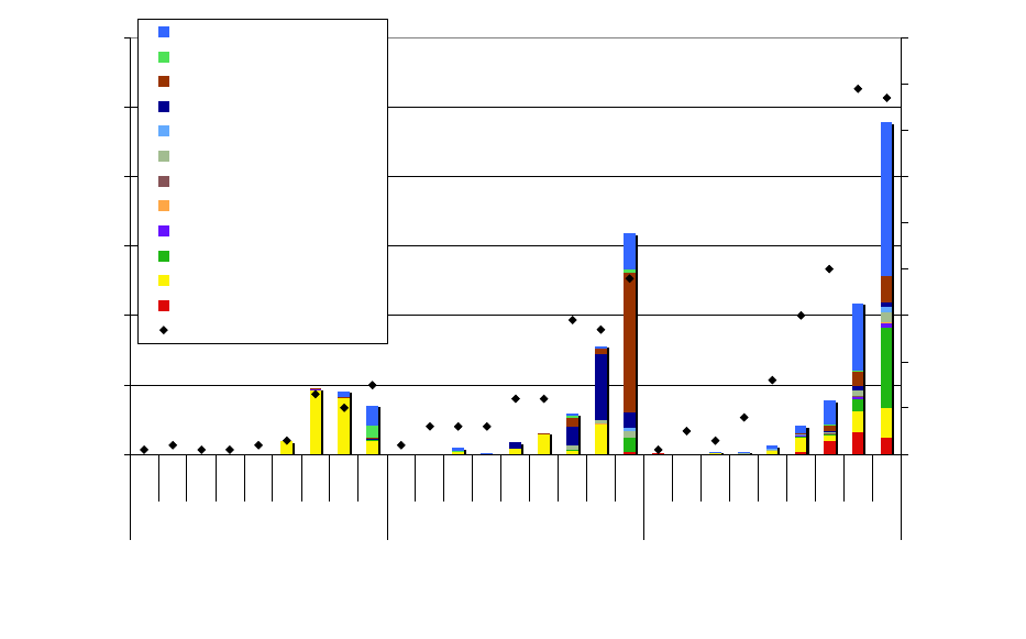
108
Figure 5.3. Global venture capital and private-equity investments by solar technology
(New Energy Finance 2009)
Private investments in Asia, almost nonexistent until 2005, have remained focused mainly on the
production of crystalline silicon PV. Private investments in Europe started somewhat earlier and
have focused on crystalline silicon PV and polysilicon production, with additional interest in
project developers and thin-film technologies in recent years. In contrast, U.S. private
investments have been broadly diversified, with investments in nearly all areas of the solar
industry and increasing interest in concentrating photovoltaics (CPV), next-generation PV,
concentrating solar power (CSP), and project developers. Most importantly, of the $1.52 billion
of global private investment that thin-film PV received in 2008, $1.11 billion went to U.S.-based
companies.
In terms of regional differences in private-equity versus venture-capital investments, private-
equity investment has been predominant in Europe. A great majority of private-equity
investment in the solar industry has been to finance capacity expansions (often by means of
constructing new factories), thus indicating that companies based in the European Union have
been building a majority of these factories. In contrast, venture-capital investment has been
predominant in the United States. Venture-capital investment is an indicator of new technologies
or business models. Whereas generous subsidy programs in the European Union have spurred
companies there to expand capacity rapidly, the market in the United States has not been
sufficiently attractive to enable significant growth of incumbent products. Therefore more U.S.
investment has been directed to innovative technologies with longer-term prospects.
$0
$500
$1,000
$1,500
$2,000
$2,500
$3,000
2000
2001
2002
2003
2004
2005
2006
2007
2008
2000
2001
2002
2003
2004
2005
2006
2007
2008
2000
2001
2002
2003
2004
2005
2006
2007
2008
Asia EU* US**
Region / Year
Millions of $
0
10
20
30
40
50
60
70
80
90
Number of Transactions
Thin Film PV
Solar Heating & Cooling
Project Developer
Polysilicon
Other
Next Generation PV
Multijunction
Manufacturing Equipment
Inverters
CSP
Crystalline Silicon PV
CPV
Number of Transactions
Source: New Energy Finance
*EU includes Israel, Morocco, & South Africa
**U.S. includes Australia and Canada
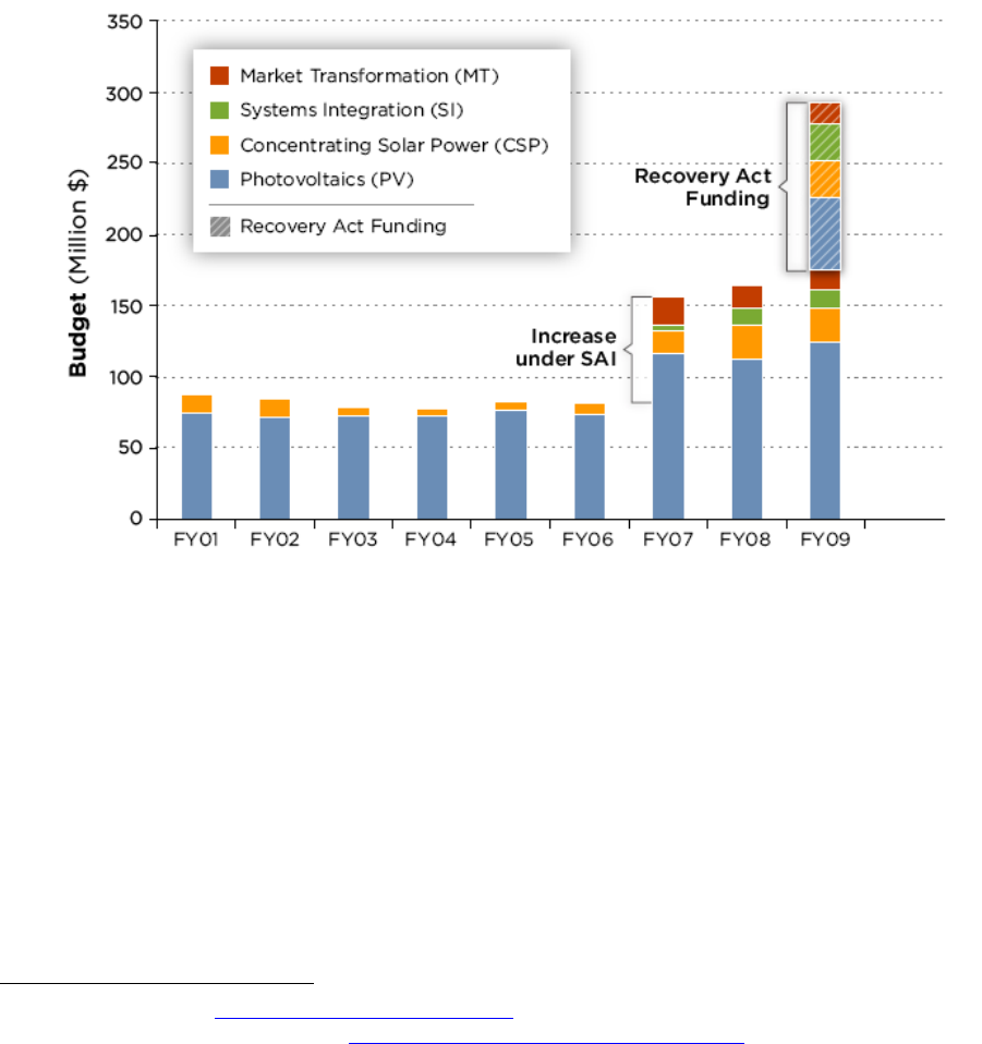
109
5.2 U.S. Department of Energy Investment in Solar Energy
The U.S. Department of Energy (DOE) Solar Energy Technologies Program (SETP)
81
plays a
key role in accelerating the development of the U.S. solar industry and the advancement of solar
technologies. SETP investments have helped foster a diverse set of technology pathways.
SETP’s long-term objective is to achieve high market penetration of solar energy technologies
with an interim goal of achieving cost parity with conventional forms of electricity by 2015 (U.S.
DOE 2009).
82
SETP efforts are implemented through four subprograms: Photovoltaics (PV),
Concentrating Solar Power (CSP), Systems Integration, and Market Transformation. The PV and
CSP subprograms focus on lowering the levelized cost of solar energy through research and
development. Systems Integration focuses on technologies, tools, and strategies to optimize the
integration of solar energy into the grid. Market Transformation addresses non-R&D barriers to
achieving high market penetration of solar energy technologies.
Figure 5.4. DOE SETP budget history from FY 2001 to FY 2009
DOE SETP FY 2007 and FY 2008 research and development budgets were $157 million and
$164 million, respectively, with the FY 2007 budget representing an increase of approximately
$75 million compared to FY 2006 (see Figure 5.4). Most of the budget increase for FY 2007, and
continuing into FY 2008, was conveyed under the umbrella of the Solar America Initiative
(SAI). In addition to increased funding for PV research and development (R&D), funding in
FY 2007 and FY 2008 provided additional resources for CSP R&D, Systems Integration, and
Market Transformation. In FY 2008, funding allocated to the four subprograms was $112 million
for PV, $24 million for CSP, $12 million for Systems Integration, and $16 million for Market
Transformation. In FY 2009, the SETP budget increased again, to $175 million, comprised of
$125 million for PV, $24 million for CSP, $12 million for Systems Integration, and $14 million
for Market Transformation. In addition, the American Recovery and Reinvestment Act of 2009
81
DOE SETP Web site: http://www.eere.energy.gov/solar/
82
DOE SETP FY 2008 Annual Report: http://www.nrel.gov/docs/fy09osti/43987.pdf.

110
provided nearly$118 million
83
The majority of SETP funding is directed at cost-shared research, development, demonstration,
and deployment efforts with national laboratories, states, industry, and university partners. For
current, upcoming, and past funding opportunities in all research areas, see:
in additional funds to SETP, bringing the total FY 2009 budget to
$293 million. Recovery Act funding in FY 2009, as allocated to the subprograms, was $52
million for PV, $26 million for CSP, $26 million for Systems Integration, and $15 million for
Market Transformation.
http://www.eere.energy.gov/solar/financial_opportunities.html.
The DOE SETP Photovoltaics subprogram
84
The Concentrating Solar Power subprogram
invests in technologies across the development
pipeline that demonstrate progress toward minimizing the effective life-cycle cost of solar
energy. The PV subprogram’s activities are organized into three focus areas: new devices and
processes, prototype design and pilot production, and systems development and manufacturing.
Highlights in FY 2008 were: 1) Awarded more than $65 million for 62 industry projects
spanning early-stage to market development, addressing the challenges of scaling up novel,
low-cost manufacturing for crystalline silicon, thin film, and concentrating PV technologies; and
2) Achieved world-record efficiencies through applied research at the national laboratories,
including a 20.0%-efficient CIGS thin-film PV device and a 40.8%-efficient inverted
metamorphic multijunction solar cell.
85
The Systems Integration subprogram
has been ramping up R&D and deployment efforts
in recent years, leveraging industry partners and the national laboratories. The CSP subprogram
aims to increase U.S. deployment of CSP, achieve intermediate power market competitiveness
by 2015, and develop advanced technologies to reduce system and storage costs, enabling base-
load power market competitiveness by 2020. R&D activities focus on linear concentrator
systems such as parabolic troughs and linear Fresnel reflectors, dish-engine systems such as
dish/Stirling engine systems, thermal storage systems and advanced heat transfer fluids,
advanced concepts R&D, and CSP market transformation. Highlights in FY 2008 were:
1) Established 15 partnerships with universities and CSP companies to support innovations in
advanced high-temperature, heat-transfer fluids and thermal storage systems; and 2) Partnered
with the Bureau of Land Management to initiate a Programmatic Environmental Impact
Statement and conducted other joint activities necessary for the development of federal land in
the Southwest for utility-scale solar projects (also see Section 2.4.5, Land and Transmission
Constraints for Utility-Scale Solar).
86
83
The exact Recovery Act funding level was $117.6 million.
focuses on breaking down the regulatory, technical, and
economic barriers to integrating solar electricity into the electric grid by developing technologies
and strategies in partnership with utilities and the solar industry. Systems Integration R&D
includes Solar System Technology Development, Advanced Systems Integration, System
Testing and Demonstrations, Renewable Energy System Analysis, Solar Resource Assessment,
and Codes, Standards and Regulatory Implementation. Highlights in FY 2008 were: 1) Awarded
funds to 12 industry teams through the Solar Energy Grid Integration Systems project to develop
84
DOE SETP PV subprogram Web site: http://www.eere.energy.gov/solar/photovoltaics_program.html
85
DOE SETP CSP subprogram Web site: http://www.eere.energy.gov/solar/csp_program.html
86
DOE SETP Systems Integration subprogram Web site:
http://www.eere.energy.gov/solar/systems_integration_program.html.
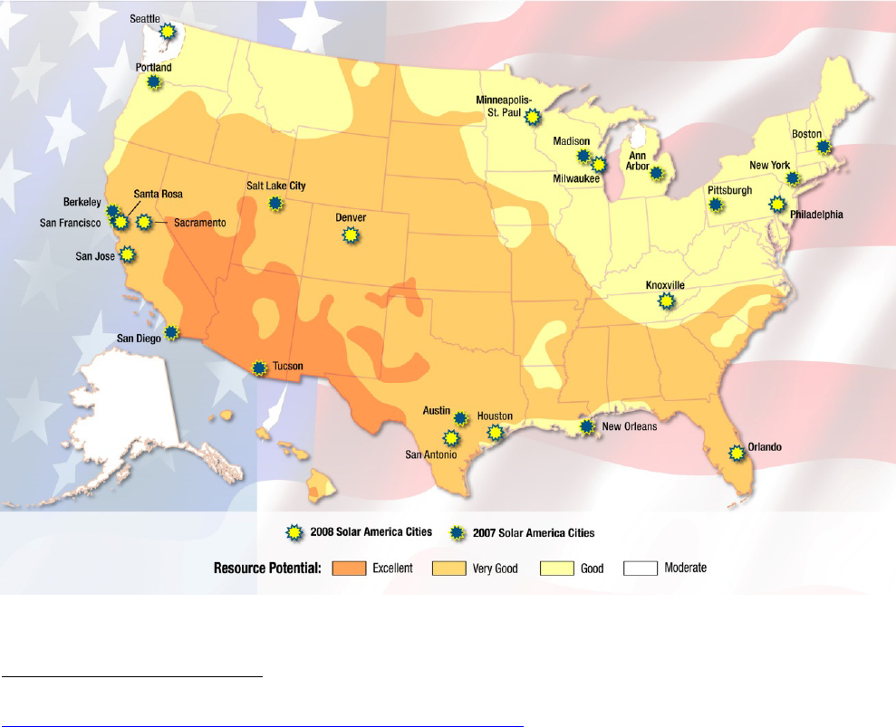
111
new inverters and controllers with interfaces to energy-management systems; and 2) Established
monitoring of large-scale PV performance at high-penetration sites in California, Colorado, and
Hawaii to better understand how high levels of PV impact the grid and reduce installation costs.
The Market Transformation subprogram
87
promotes the commercialization of solar technologies
by addressing non-R&D barriers to solar energy adoption. Activities include codes and standards
development, outreach to state and utility decision makers, workforce development, solar
installation technical assistance, and the Solar America Cities program. DOE partners with
several organizations including the Solar America Board for Codes and Standards, the Solar
Electric Power Association, the Interstate Renewable Energy Council, the National Association
of Regulatory Utility Commissioners, the National Conference of State Legislatures, and the
Clean Energy Group. Highlights in FY 2008 were: 1) Strengthened the responsiveness,
effectiveness, and accessibility of PV codes and standards through the Solar America Board for
Codes and Standards, including release of three studies on interconnection procedures for utility
regulators, solar access laws, and external disconnect switches; and 2) Expanded the Solar
America Cities program from 13 to 25 partnerships, to further accelerate deployment of solar
energy technologies by providing financial and technical assistance to cities committed to
making solar a mainstream energy source (Figure 5.5).
Figure 5.5. 2007 and 2008 Solar America Cities
87
DOE SETP Market Transformation subprogram:
http://www.eere.energy.gov/solar/market_transformation_program.html
.

112
5.3 Solar Market Forecasts, PV and CSP
5.3.1 PV Market Forecasts
The recent expansion of the PV market has prompted numerous analysts from financial
institutions and research and consulting firms to provide analysis and forecasts for the PV sector.
This section analyzes these projections, both to identify the expected path of the industry and to
recognize the substantial variance in market forecasts. Key trends and uncertainties for the PV
market in the next several years also are discussed.
The global economic crisis that became apparent in late 2008, and which is expected to diminish
funds available for investments and reduce the demand for PV, caused some analysts to revise
their forecasts substantially in reports released in early 2009 compared to forecasts released in
mid-to-late 2008. This section focuses on the projections made in early 2009. For a detailed
discussion about the effects of the economic crisis on PV forecasts, see the full report from
which the data and discussion in this section have been extracted (Bartlett et al. 2009).
88
Figure 5.6 illustrates the forecasted size and composition of PV production through 2012. For
total production, the median estimate increases from 5.6 GW in 2008 to 21 GW in 2012, a 4-year
CAGR of 40%. For both the c-Si and thin-film PV segments, the growth is expected to be
greatest through 2010, with growth slowing somewhat in 2011 before accelerating again in 2012.
In addition to the growth of the median estimate, the range of estimates is significant. In 2012,
the high estimates for c-Si and thin film are roughly three times as great as the low estimates.
These uncertainties are due to different opinions about the demand for PV modules, the ability to
expand production sufficiently for each part of the PV supply chain, and the technological and
cost improvements of c-Si.
88
The Effects of the Financial Crisis on Photovoltaics: An Analysis of Changes in Market Forecasts from 2008 to
2009:
www.nrel.gov/docs/fy10osti/46713.pdf
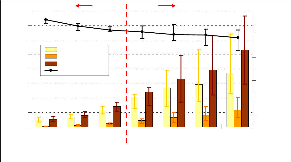
113
Figure 5.6. Global total PV module production forecasts
(Mehta and Bradford 2009, Citi Investment Research 2009, Cowen & Co. 2009,
Deutsche Bank 2009, Lazard 2009, Morgan Stanley 2009, Mints and Tomlinson 2008,
Mints 2009, Chase et al. 2009, Thomas Weisel 2009)
Regarding thin-film versus c-Si production, thin-film production is expected to grow faster than
c-Si production during the next several years, with a forecasted 2008–2012 CAGR for thin-film
PV of 52% versus 33% for c-Si PV. However, c-Si is still expected to be the dominant
technology for the next several years, accounting for about 77% of total PV production in 2012.
There is, however, considerable disagreement among analysts about the future PV market share
of c-Si versus thin film; the 2012 c-Si market share estimates range from 66% to 84%.
To better describe the thin-film sector, Figure 5.7 presents the projected rise in thin-film PV
module production by technology through 2010. The range of supply estimates (i.e., the
considerable uncertainty) for thin-film PV is reasonable given that thin film faces technology and
scale-up risks in addition to overall PV market uncertainty. Despite the uncertainty, tremendous
growth is implied by the median estimates, with 2008–2010 CAGRs of 70% for CdTe, 85% for
a-Si, and 96% for CIGS production.
For CdTe, First Solar accounts for virtually all the 2008 CdTe production of roughly 0.50 GW,
and the company plans to have 1.1 GW of manufacturing capacity by the end of 2010. The
uncertainty in the 2009 and 2010 production estimates might result from divergent opinions
regarding the prospects of new CdTe entrants, such as PrimeStar Solar and Abound Solar, as
well as uncertainty regarding the pace of First Solar’s expansion.
For a-Si, there are established producers such as Energy Conversion Devices, Sharp, and
Kaneka, as well as numerous new entrants, many of which have planned to enter the market
through the purchase of turnkey systems from Applied Materials or Oerlikon. However, given
the capital expenditures necessary for the purchase of turnkey production lines, expansion of a-Si
0
4
8
12
16
20
24
28
32
2006 2007 2008 2009 2010 2011 2012
Ye ar
PV Production (GW-dc)
0%
10%
20%
30%
40%
50%
60%
70%
80%
90%
100%
c-Si Market Share (%)
c-Si
Thin Film
Total
c-Si market share
Low
Median
High
HIST ORICAL
PROJ EC T ED
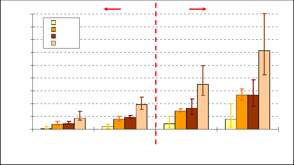
114
production from new entrants has been curtailed by the tight credit environment. In addition, as
PV module prices have fallen faster than system prices over the past year, non-module costs have
risen as a proportion of total system costs. Because non-module costs per watt rise as module
efficiency declines, a-Si (which has the lowest efficiency of any of the principal PV
technologies) has become less attractive.
CIGS module production is starting from a very low base, a median 2008 estimate of just
0.10 GW, but is expected to grow substantially in the near term. The median projection for 2010
is 0.40 GW, with a low estimate of about 0.10 GW and a high estimate of about 1.0 GW. The
enormous range reflects the substantial scale-up and technology risks as companies such as
Miasole, Nanosolar, and Solyndra expand commercial production.
Figure 5.7. Global thin-film PV module production forecasts
(Mehta and Bradford 2009, Citi Investment Research 2009, Deutsche Bank 2009,
Lux Research 2009)
Figure 5.8 shows the demand projections for solar PV modules by location. Global demand is
expected to grow from 5.8 GW in 2008 to 19 GW in 2012, a 4-year CAGR of approximately
34%. Europe, with Germany continuing to be the dominant market in the continent, is expected
to remain the largest region for solar power. However, the North American market is expected to
grow the fastest. Four-year CAGRs are 14% for Europe, 87% for North America, 39% for Japan
and South Korea, and 50% for the rest of the world (ROW). As with the production projections,
there is tremendous range in the demand estimates resulting from the uncertainty about policy
incentives, electricity prices, cost reductions of PV systems, and the price elasticity of PV
demand.
The United States is expected to account for a large majority of North American demand through
2012. However, analysts also expect Canada to contribute meaningfully, particularly as a result
0.0
0.5
1.0
1.5
2.0
2.5
3.0
3.5
4.0
4.5
2007 2008 2009 2010
Ye ar
PV Production (GW-dc)
CIGS
a-Si
CdTe
Total
Low
Median
High
HIST ORICAL
PROJEC T ED

115
of Ontario’s enhanced feed-in tariff. Mexico and other North American countries are not
expected to contribute substantially to PV demand in the near term.
Figure 5.8. Global PV module demand forecasts
(Barclays 2009, Citi Investment Research 2009, Cowen & Co. 2009, Lazard 2009,
Morgan Stanley 2009, Oppenheimer 2009, Thomas Weisel 2009, UBS 2009)
Figure 5.9 shows forecasted global module and system prices through 2010. Module prices are
expected to decrease from $3.72/W in 2008 to $2.45/W in 2010, a 2-year CAGR of –18.8%.
System prices are expected to decrease by a slightly smaller proportion, from $6.08/W in 2008 to
$4.21/W in 2010, a 2-year CAGR of –16.8%. By comparison, the average U.S. PV system cost
was $7.50/W in 2008. Although estimated non-module prices cannot be calculated directly from
Figure 5.9 (some analysts forecast only system prices and others forecast only module prices), it
is likely that the module prices are expected to decline faster than non-module prices through
2010. This is not surprising given the previous supply shortages that have kept PV module prices
from declining over the last few years despite cost improvements. Thus, there is significant room
for price declines within the PV-module cost structure.
0
2
4
6
8
10
12
14
16
18
20
22
24
26
2006 2007 2008 2009 2010 2011 2012
Ye ar
PV Demand (GW-dc)
Rest of world
Japan & S Korea
North America
Europe
Total
Low
Median
High
HIST ORICAL
PROJ EC T ED
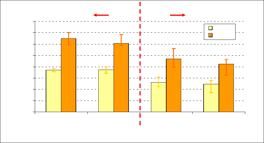
116
Figure 5.9. Global PV module and system price forecasts
(Cowen & Co. 2009, Deutsche Bank 2009, Deutsche Bank 2009a, Lazard 2009,
Lux Research 2009, Morgan Stanley 2009, UBS 2009)
5.3.2 CSP Market Forecasts
CSP differs markedly from PV with respect to history, installation size, permitting and
construction duration, and technological readiness. Whereas PV has had a history of consistent
annual installations, 350 MW of CSP were built in the 1980s with no subsequent installations in
the United States until 2005. Installation sizes on the order of tens of megawatts, and up to
4-year permitting and construction durations, contribute to the difference in deployment patterns
between CSP and PV. Finally, only one CSP technology (parabolic troughs) has been
demonstrated long term on a fully commercial scale. As of mid-2009, two power towers were
grid-tied in Spain, but this technology type is still relatively new to the commercial market. In
addition, dish-engine systems and linear Fresnel reflectors have not yet been deployed at a near-
commercial scale. For these reasons, the scope of CSP forecasting is more limited.
Tables 5.1 and 5.2 list the amount and location of planned CSP installations through 2015; these
include systems that have been commissioned, financed, under construction, announced, or
proposed (Bullard and d’Avack 2009). Of the more than 12 GW in the CSP pipeline, more than
50% is in the United States, 33% is in Spain, about 8% is in the Middle East and North Africa
(MENA) region, and the remaining 8% is dispersed across Australasia, Europe, and the Republic
of South Africa. It should be noted that the projects in the global pipeline are by no means
guaranteed. Several major factors could prevent many of these projects from being completed,
resulting in a pipeline that will likely be reshaped on a continual basis.
Table 5.3 shows the U.S. CSP power purchase agreement (PPA) pipeline market shares by
technology, based on about 4.3 GW of PPAs (two-thirds of the 6.5 GW in the U.S. pipeline
shown in Table 5.1). In contrast to CSP installed and under construction (see Section 1.3), which
is dominated by parabolic trough technology, troughs and towers are equally represented in the
U.S. PPA pipeline.
$0.00
$1.00
$2.00
$3.00
$4.00
$5.00
$6.00
$7.00
$8.00
2007 2008 2009 2010
Ye ar
Average Selling Price ($/W-dc)
Module
System
Low
Median
High
HIST ORICAL
PROJEC T ED
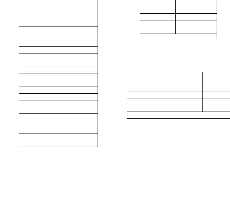
117
Table 5.1. Global CSP Planned Projects,
Capacity by Country, Through 2015
Country
Capacity
(GW)
United States
6.5
Spain
4.2
India
0.46
Jordan
0.40
Israel
0.40
Italy
0.11
China
0.10
U.A.E
0.10
South Africa
0.10
Australia
0.083
Greece
0.062
Mexico
0.052
Oman
0.050
Egypt
0.030
Algeria
0.025
Morocco
0.020
France
0.012
Chile
0.010
Total
12.7
Bullard and d’Avack 2009
Table 5.2. Global CSP Planned Projects,
Market Share by Country, Through 2015
Country
Market Share
United States
51%
Spain
33%
MENA
8%
ROW
8%
Bullard and d’Avack 2009
Table 5.3. U.S. CSP Power Purchase
Agreement Pipeline, Market Share by
Technology, Through 2015
Technology
Capacity
(GW)
Market
Share
Parabolic trough
1.8
41%
Tower
1.7
40%
Dish-engine
0.83
19%
Total
4.3
Bullard and d’Avack 2009
5.4 References
Barclays Capital. (2009). Solar Energy Handbook: The Second Growth Phase of Solar Era.
Barclays Capital.
Bartlett, J.E.; Margolis, R.M.; Jennings, C.E. (2009). The Effects of the Financial Crisis on
Photovoltaics: An Analysis of Changes in Market Forecasts from 2008 to 2009. National
Renewable Energy Laboratory. Technical Report NREL/TP-6A2-46713.
http://www.nrel.gov/docs/fy10osti/46713.pdf. Accessed September 2009.
Bullard, N.; d’Avack, F. (June 23, 2009). STEG Revolution III: Still Steaming. Research Note.
London: New Energy Finance.
Chase, J.; Wu, J.; d’Avack, F.; Bullard, N.; Simonek, M.. (March 31, 2009). PV Market Outlook:
It’s Darkest Before the Dawn. Research Note. London: New Energy Finance.
Citi Investment Research. (2009). U.S. Solar Stocks: Inventory Has Yet to Peak, so It’s Still Too
Early. Citi Investment Research.
Cowen & Co. (2009). Industry Outlook: Industry Hoping for Help from Stimulus Bill. Cowen &
Co.
Deutsche Bank. (2009). Solar Photovoltaic Industry: Looking Through the Storm. Deutsche
Bank.
Deutsche Bank. (2009a). Personal communication.

118
Lazard. (2009). A Framework for Assessing Solar Stocks in Turbulent Times. Lazard Capital
Markets.
Lux Research. (2009). Finding the Solar Market’s Nadir. Lux Research.
Mehta, S.; Bradford, T.; (January 2009). PV Technology, Production, and Cost, 2009 Forecast:
The Anatomy of a Shakeout. Greentech Media, Inc., and the Prometheus Institute.
Morgan Stanley. (2009). Solar Devices: Dislocation – Industry Reset. Morgan Stanley.
Mints, P.; Tomlinson, D. (2008). Photovoltaic Manufacturer Shipments & Competitive Analysis
2007/2008. Report # NPS-Supply3. Palo Alto, CA: Navigant Consulting Photovoltaic Service
Program.
Mints, P. (2009). Photovoltaic Manufacturer Shipments, Capacity, & Competitive Analysis
2008/2009. Report # NPS-Supply4. Palo Alto, CA: Navigant Consulting Photovoltaic Service
Program.
New Energy Finance (2009). New Energy Finance Desktop 3.0. www.newenergymatters.com.
Accessed May 20, 2009.
Oppenheimer & Co. (2009). PV Market Forecast. Oppenheimer & Co.
Thomas Weisel Partners. (2009). Alternative Energy; Presentation Materials to Investors.
Thomas Weisel Partners.
U.S. DOE. (2009). DOE Solar Energy Technologies Program. FY 2008 Annual Report.
http://www.nrel.gov/docs/fy09osti/43987.pdf. Accessed August 2009.
UBS. (2009). Darwin’s Theory – Survival of the Fittest. UBS Investment Research.

Solar Energy Web Sites
U.S. Department of Energy, Solar Energy Technologies Program
www.solar.energy.gov
U.S. Department of Energy, Solar America Cities Web site
www.solaramericacities.energy.gov
National Renewable Energy Laboratory (NREL) Solar Energy Technologies Program
www.nrel.gov/solar
National Renewable Energy Laboratory (NREL) Energy Analysis
www.nrel.gov/analysis
Sandia National Laboratories (SNL) Solar Technologies Department
www.sandia.gov/solar
Lawrence Berkeley National Laboratory (LBNL) Electricity Markets and Policy
eetd.lbl.gov/EA/EMP/emp-pubs.html
Database of State Incentives for Renewables and Eciency (DSIRE)
www.dsireusa.org
Interstate Renewable Energy Council (IREC)
irecusa.org
Solar Energy Industries Association (SEIA)
www.seia.org
Solar Electric Power Association (SEPA)
www.solarelectricpower.org
American Solar Energy Society (ASES)
www.ases.org
Key Report Contacts
For more information on this report, please contact:
Selya Price, National Renewable Energy Laboratory
202-488-2205, Selya.Price@nrel.gov
Robert Margolis, National Renewable Energy Laboratory
202-488-2222, Robert.Margolis@nrel.gov
On the Cover
(Main photo) At more than 8 MW of nameplate capacity, the photovoltaic (PV) power plant near Alamosa, Colorado, is one of the largest
in the United States. The Alamosa plant came online in December 2007 through a partnership between SunEdison and Xcel Energy.
– Courtesy of Zinn Photography and SunEdison/PIX 15563
(Insert) The Nevada Solar One concentrating solar power (CSP) plant near Boulder City, Nevada, is a 64 MW parabolic trough installation
completed in June 2007 by developer Acciona Energy.
– Courtesy of Acciona Energy Corporation/PIX 15996
For more information contact:
EERE Information Center
1-877-EERE-INF (1-877-337-3463)
www.eere.energy.gov/informationcenter
Printed with a renewable-source ink on paper containing at
least 50% wastepaper, including 10% post consumer waste.
Prepared by the National Renewable Energy Laboratory (NREL)
NREL is a national laboratory of the U.S. Department of Energy
Office of Energy Efficiency and Renewable Energy
Operated by the Alliance for Sustainable Energy, LLC
DOE/GO-102010-2867
January 2010
Energy Efficiency &
Renewable Energy
